In The Name of God

Analytic Computational Statistical Data Compression

Abstract: A new statistical algebraic method for data compression is presented. The method is expected to compress Data more than 1/10000. In fact, the more our computation power is, the more we are able to compress. Some other methods like the irrational number method and geometric method are presented. But the focus of the article is on the statistical method.

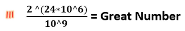
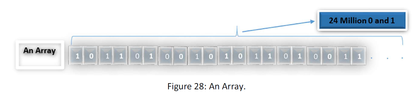
Idea Explanation: suppose a kind of data element has 3 MB volume. 3 MB can depict 2^ (24*10^6) arrays of 0,1. All the frames we have built and will build is, for instance, 2^1000 frames. (at most this will be 2^100, but we assume 2^1000). Anyway, this is obvious that all the frames we work with in practice are a very small amount of all probable 0,1 arrays in 1 MB. Suppose that we have gathered all those 2^1000 frames. This number related to all the arrays in 1 MB is the ratio of 1/2^ (23*10^6 +999000). This is approximately nothing. As mentioned before, our fundamental challenge in compressing data is that the number of possible arrays of 0,1 is not equal to two amount of data, for instance in 1 MB and 1GB. Thus this is not possible to find a one to one map in their arrays space. But, what if we know that all our data that we are dealing with is restricted in a space in the arrays space? If there is so, we can find a map or literature that only map that limited space to another less heavy space. For instance, a map from 1 GB to 1 KB. illustrating more the idea, firstly I need to introduce some spaces for this purpose.

Step One: Building Space

Each array can be represented as a number. For instance, the array 100000… is 1, the array 01000000… is 2, And so on. (There are different ways to map the arrays to natural number set. The one proper for our purpose is one that compact the data most that we discuss in the section “conversions”.) Then we can build some spaces in this arrays. The 1 D space is so that we arrange these arrays in a line.  

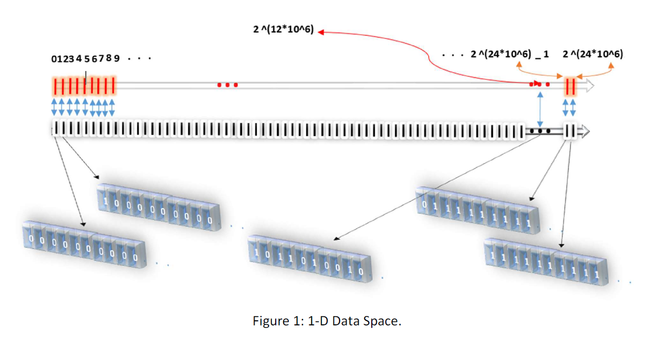
The 3D space is a space that the first dimension is the arrays consist of 3N+1 numbers of each possible arrays and the second dimension is the arrays consist of 3N+2 numbers of each possible arrays and the third dimension is the arrays consist of 3N+3 numbers of each possible arrays another dimension is the odd numbers. Each array would be like this:

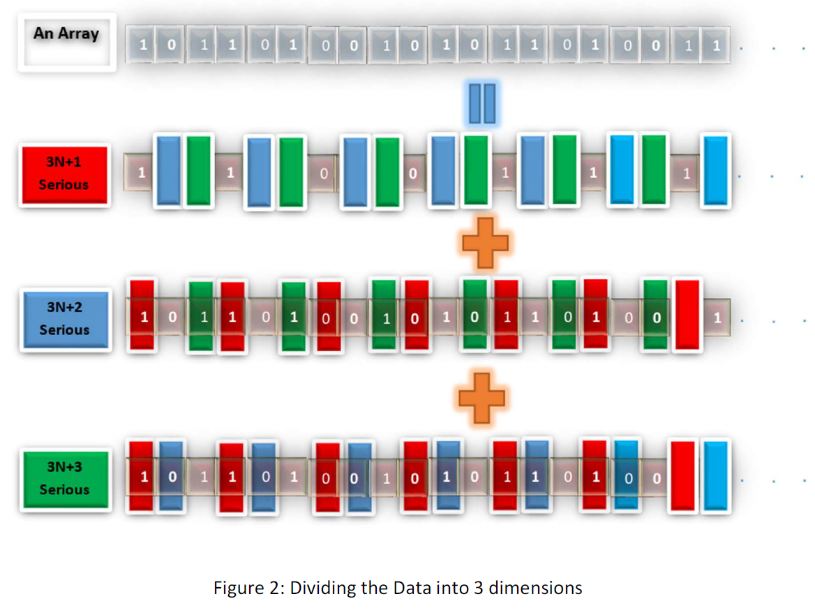
Then for each possible array, we have a 3N+1 serious and a 3N+2 serious and 3N+3 serious each one with 1/3 length of the array as follow:

S = T1(s) + T2(s) + T3(s)

(we could build 2D, 4D or any dimension space. But for the proper illustration I use 3D dimension) 

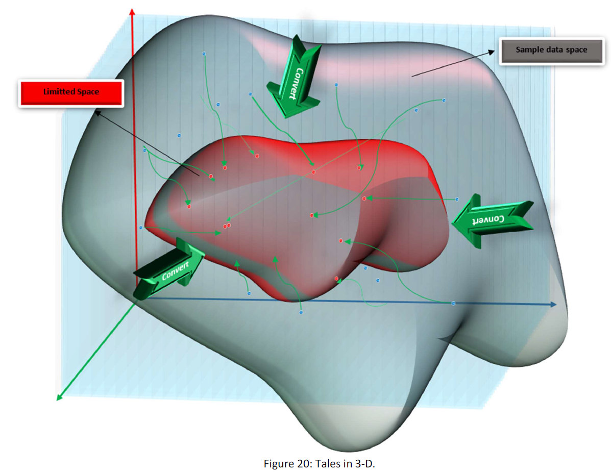
For each 3MB array, there are a T1, T2, and T3 series and their combination is the array and the triple (T1, T2, T3) for the array is unique. Also for each serious in T1, T2, and T3, there is a number in N (natural numbers set). Consequently, there is a one-to-one map between the field N^3 and the field         ( T1 ,T2 ,T3 ). Then for each possible array t,here is a point in 3D discrete  space or N^3.  Then we have a 3D discrete space that each point in the space is a possible array of 3MB data. Suppose the following figure:

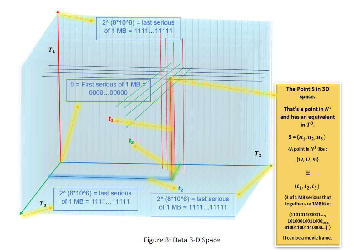
Each point in the space is the equivalent to 3 of 1 MB series and thus equivalent to a 3MB array. The space contains all possible arrays of volume 3 MB. For instance, a movie frame is a point in the space. 

An important point is that space is not continuous, but discrete. That the points of the space are finite and equal to the possible arrays contained in 3 MB. 

Step2: Gathering Samples

(Space of 3MB possible arrays in 1D) We sample 10 billion frames from different types of frames randomly. Then we scattered the codes in our space; for instance, 3D space. (as we can. The number of samples we need may determine through some evaluation that is no a concern of the article) Each code is like a point in the space. 

Then there are two probable situations we may meet:

1) Limited Samples: The codes are located in the specific part of the space.

2) Scattered Samples: The codes are distributed in whole the space.

First I investigate the situation that the codes are located in the limited space.

1) Limited Samples

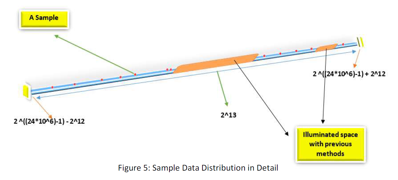
 In this condition, this is easy to find a less heavy map or a good compression. Remember that our challenge was that for each point in the larger amount of data there is not one point in the less heavy amount of Data or there is not a one-to-one map between the two space, for instance, between 1 GB and 1 KB. But if we know the space in a larger space the codes are restricted, we can only map the lesser space to only that part of the larger space. We know that for instance, in 1D space, our codes are distributed as follow:

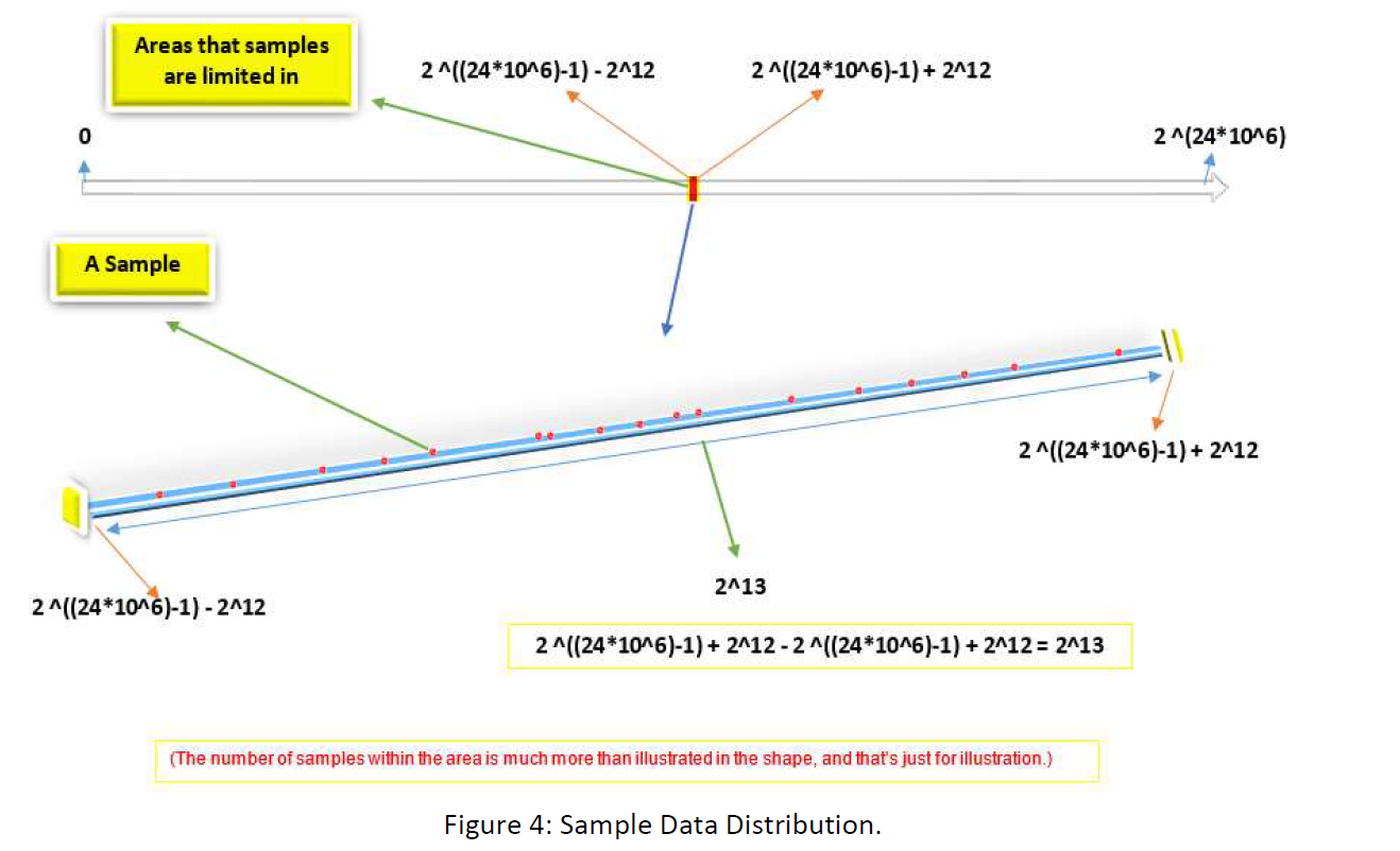
In this way, may we can compress the 3MB frame to less than 1KB. May you ask, if we suppose that those random sample frames are limited in part of the space, why the next one has to be so?  In response, I would say you are right and more professionally in philosophy, David Hume believed the same as you. There is no guarantee that the nature tomorrow behaves the same as it did yesterday. But this point also is mentionable that whole science is based on this principle that, “nature behaves in the ordered predictable way through time” and without the principle, we can’t rely on any of our empirical sciences like physics, or chemistry. Anyway, if our 10 Billion samples behave in an order, this is reasonable to assume that they all will behave so. There is another base for believing that they must be regular and ordered and that is because they are all that has come out from a human mind and must be understood by the human mind. They are all built by some limited instruments and so on. There are many hidden regularity and orders hidden in these facts that gives our data and codes the same characteristics. The previous methods are attempts to find these orders surging the data, that may be hidden in finding the space those data are limited in. For instance, they would have tried to discern some orders and then they said, the data could not be those without the order. In that way, they illuminated the space data are not in there or found the space the data restricted in. But in the method “Analytic Computational Statistical Data Compression” we do that investigation in another way and somehow in a detour. This is worthy to mention that the method doesn’t make us needless to those methods. Because the method gives us a general restriction the data is within, and maybe those methods illuminate some part of the district we obtained statistically. For instance, in the figure above, the statistical method tells us that the data is restricted within the two number  2 ^((24*10^6) -1) - 2^12 and 2 ^((24*10^6) -1) + 2^12.  But the previous method can illuminate some part of the space also like:

Another philosophical point. Our claim can be précised in the following sentence:

“The data of a Kind has an order that can be summarized or compressed.”

As if there are kinds for data and we presupposed that the data of a kind is restricted in the special part of the data space, or at least, has a special characteristic that is the kind’s characteristics.  The kind now we are talking about is movie frames. That can be any kind of data like word files, AutoCAD files etc. Any kind of data contains a set of data. Suppose the following figure:

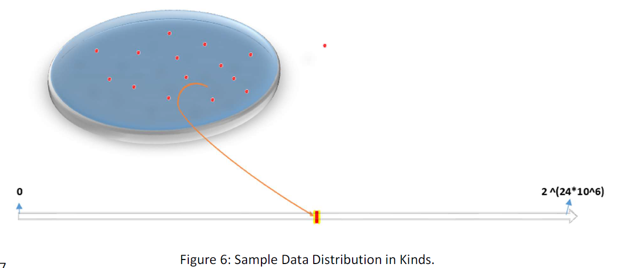
Our claim is that if a data is contained within the kind, will restrict within the part of the space.

Question: How we could know that the data is included within the corresponding kind or not?

That means, how could we know that the way we restrict the border of our kind, or we define it is the true one? 

For instance, we claim that the video files are restricted in the space (is a kind). But in practice, we get that animations are not restricted in the area. Or sad movies are not restricted in the area. More precisely, we presupposed that there are kinds that each kind is restricted in part of the space or has special characteristics. But in a realistic approach, how we know that the way we categorized the data, is the way it has distributed in the space, or the way it the data has featured in common?

This is to think realistically about the problem that, there must be an order in there that we could be able to discern that. And one can claim that there is no order there, and we just made some orders. That needn’t to an order really exist to be detected and we can make the order. 

But this is so pessimistic about the project. In this way, Newton could say how I can be sure that the Mass is a kind. That they all behave the same and obey the F = ma? Or that we consider the Horse or Human as a kind that all members of the kind must follow some rules and have characteristics and orders in common, and that’s just a guess that hasn't disappointed us so far (and sometimes has), that the kinds exist. We just follow a similar assumption in the project, this time about data.

But the matter of true categorization is an important matter that may be considered as a part of the project. Maybe kind of camera and file’s format is the fact’s that we must consider defining kinds of data. The data can be categorized somehow as follow:

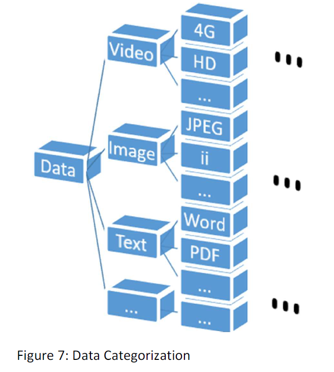
We categorize data based on our guess that the data within each categorize has special characteristics and orders that are in common in all the kind’s members.

In the end, in the best condition, we would have a map between data categorize set and the data space. Something like this:

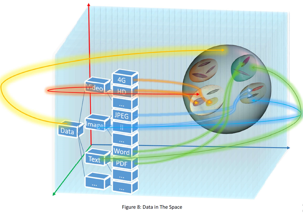
That’s a general work and that is the best condition we may meet. Anyway, that’s our purpose to find the space. In that case, we can give the data in the center of each kind of data to every receiver as a default value and then just send the distance from the data in order to transmit data. Suppose the following figure:

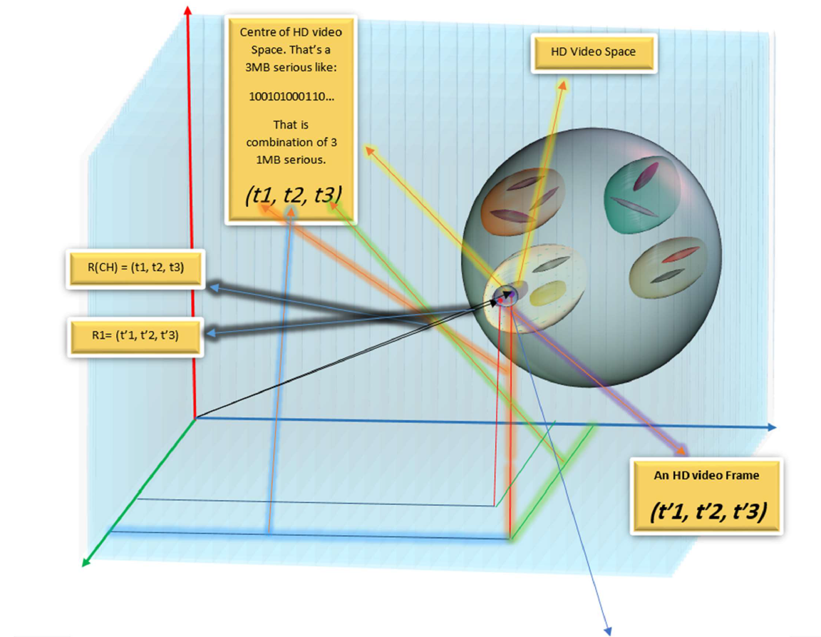
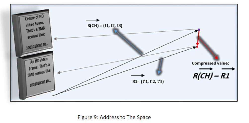
This is the way we compress data. We illuminate the value R(CH). Suppose the following figure:

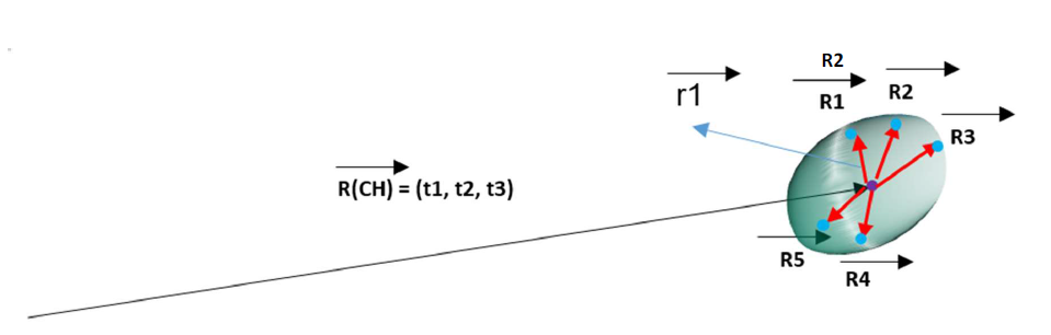
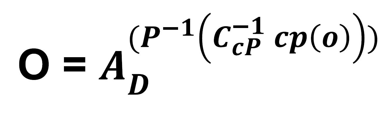
In order to address R1, R2, … we don’t need to address to them directly. Instead, first we address the area with R(CH), then we address from R(CH) to that point. In this way we have:

R1 = r1 + R(CH) 

R2 = r2 + R(CH)

R3 = r3 + R(CH) 

R4 = r4 + R(CH)

R5 = r5 + R(CH) 

As you see R(CH) is in all of them. We can give the vector R(CH) as default to the receivers and then just send the remainder r1, r2 … to them. In this way, we have illuminated the majority of the data that is R(CH) that is the great amount and though, we can compress data.

At the end though we have some kinds of data we can transmit data as follow:

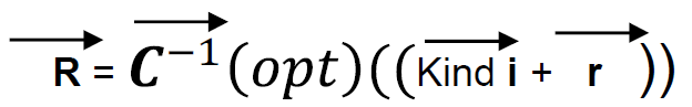
R =   r    + R(CH) 

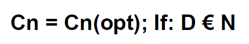
For each kind, there is an R(CH), and thus we can summarize data as:

R = Kind i + r (i= 1, 2 …n)

Kinds are known by receivers and in this way, we have compressed data.

2) Scattered Samples

We mentioned before that maybe our sample data distribution is not limited in part of the space and be scattered in whole the space.  Now I am going to talk about if we oppose this situation. In this case, we must use Conversions.

Suppose the space in 1D. In scattered samples the distribution would be something like this:

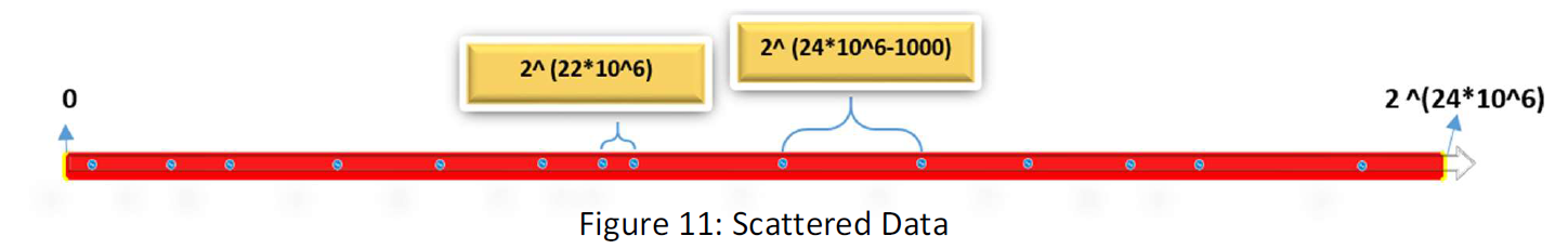
Suppose that we have 10 billion samples scattered in 1D space. Still, the distance between each two sample will be so high. If the distance between every two samples in all the sample is equal, the distance will be:

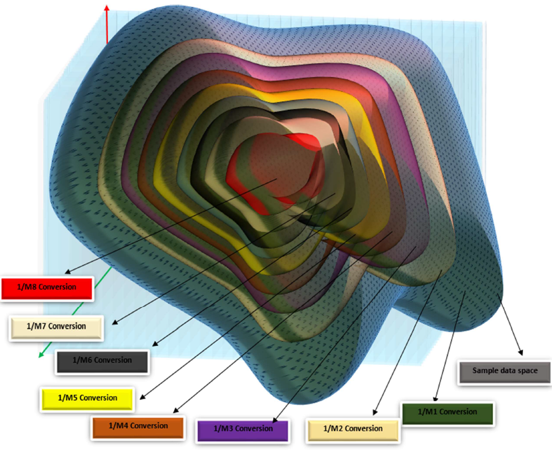
Conversion

If the samples are scattered throughout the space, we use conversions to make them limited in a tiny fraction of the space. 

What is conversion?

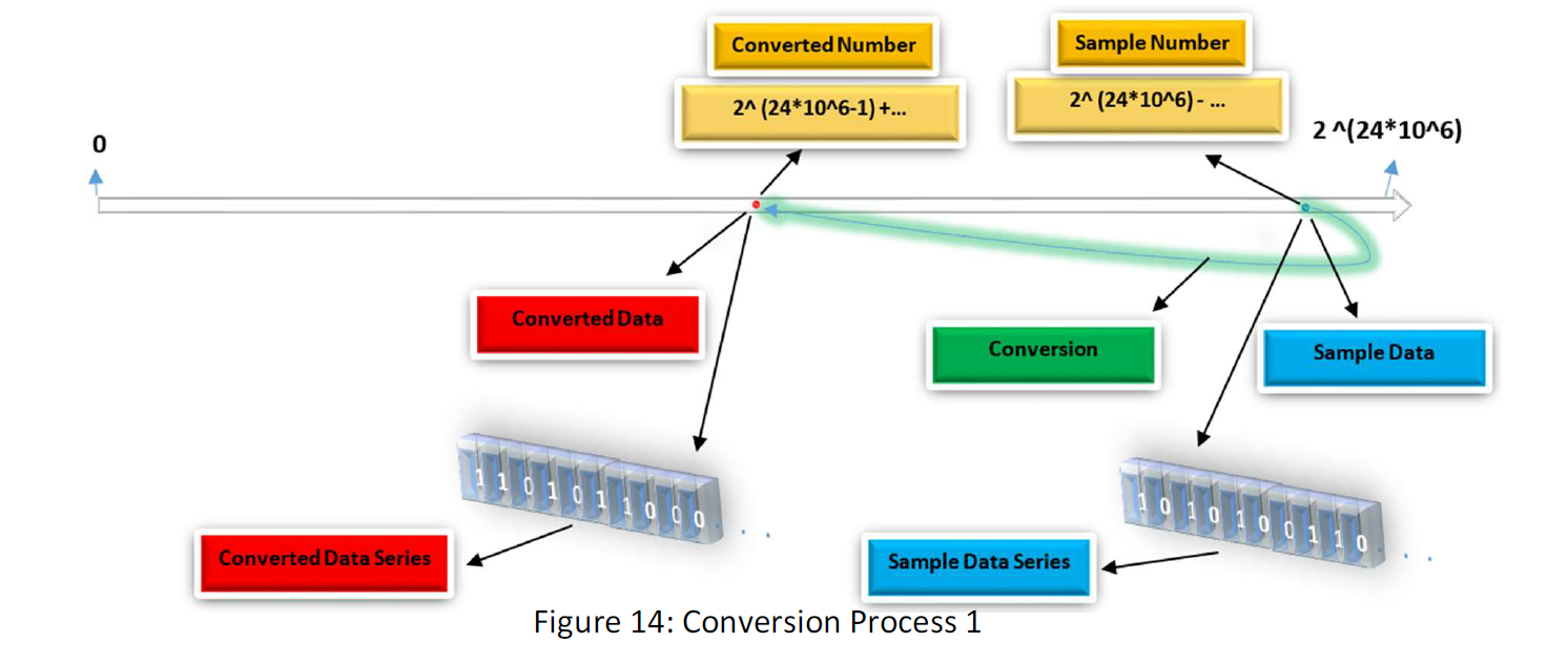
Conversion works like a function for the series. Suppose the following figure:

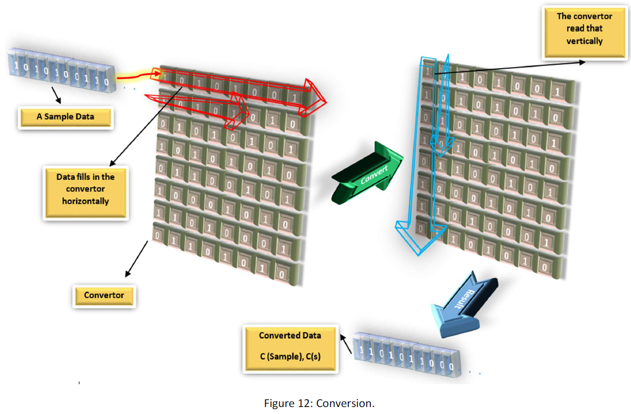
As you see, a sample goes into the converter and another data will come out. We write it so:

That C(s) is the converted data corresponding to sample s through conversion C. 

Also, we can define the negative conversion  as follow:

 is the converter that if you put converted data in; gives you the initial data. 

There are infinite possible conversions. For instance, you can change the dimension of the rectangle above or use another shape. Suppose following conversions:

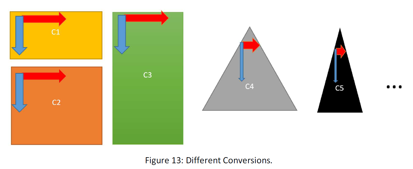
For each of the above conversions, there can be defined a negative conversion .

We can accumulate the conversions also as:

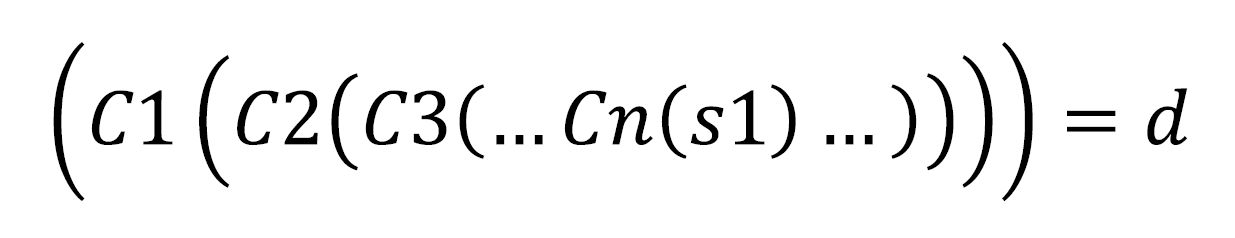
And the negative conversion will be so:

Each set of conversions gives us another conversion with a negative conversion as follow:

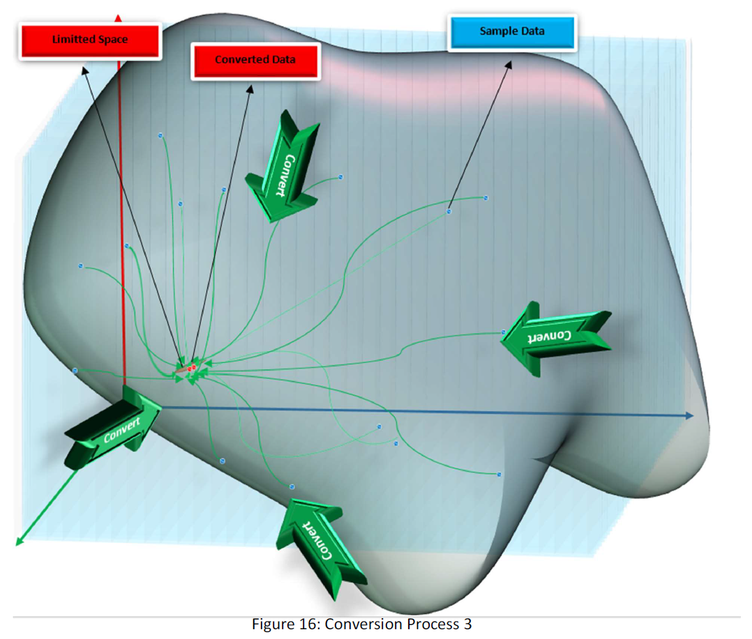
Each conversion will change the place of a data in the field of data or equivalently changes its number. Suppose the following figure:

If we put all of our samples into a conversion, then the distribution of our sample data within our data space will change. Our purpose is to find the conversion that limits the data in the smaller space as small as possible. Suppose the following figure:

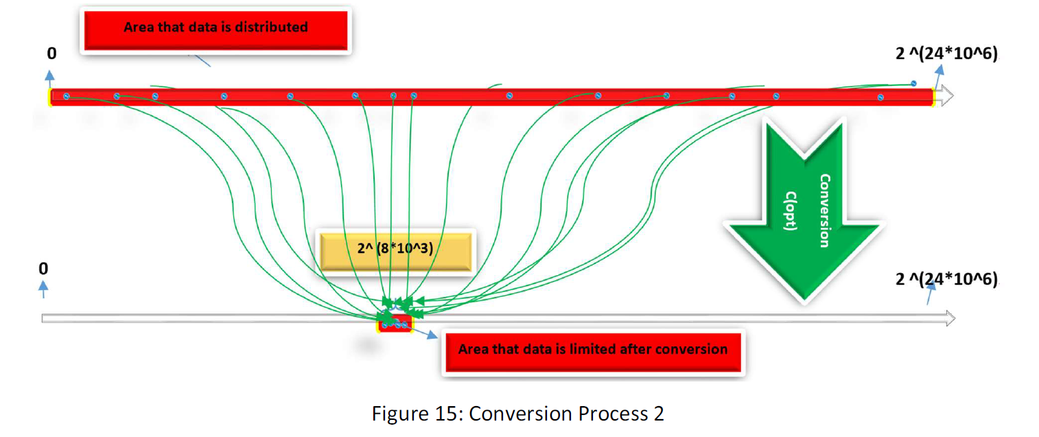
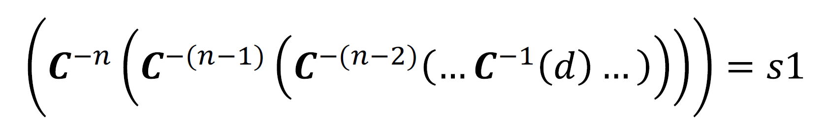
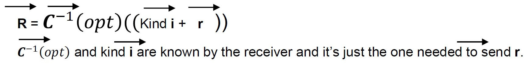
If we could find the true conversion (C(opt)), converted data are like the limited samples. We assume that if conversion limits our sample within part of the space, about all the data will do so. Thus we write:

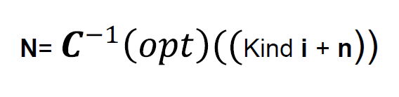
 and kind i are known by the receiver and it’s just needed to send n. 

In 3D also the procedure is the same and just a conversion in 3D is a combination of 3 conversions like this: 

And true conversion in 3D  is one that limits the data in the small part of the space as small as possible like the following figure:

Then for 3D space, we write:

The question is how to find the true conversion?

I suggest three methods for finding the C(opt). But the question worth is investigated individually in another article.

Method 1: Tales Method

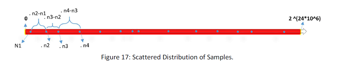
In 1D suppose that the distribution is as follow:

The number of samples is:

n1, n2, n3 …

And the distance between the numbers is

n2-n1, n3-n2, n4-n3 …

Now suppose that we divide the distances to a number like M.  Then the distances will be:

(n2-n1)/M, (n3-n2)/M, (n4-n3)/M …

And the numbers will be:

N1, N1+(n2-n1)/M, N1+ (n3-n1)/M, N1+(n4-n3)/M …

And though the samples compress near the first sample N1 as follow:

But there is a problem. Though space is discrete and not continuous, if we divide all the samples distances to number M, it is possible that many of the numbers locate between the natural numbers and have a value in R (real number set) and not N, (the natural number set).  Suppose the following figure:

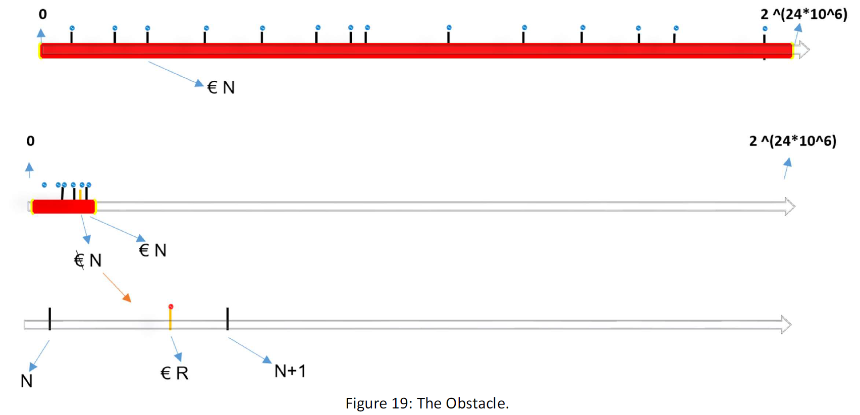
That a converted serious or value don’t be in set N, means that the conversion is not working. In continuous space (R) each part of space can map 1-to-1 to another part of the space, by any relative magnitude. because the cardinal of all Sets in R is equal to each other. 

But we work with finite sets that one is bigger than the other and the sets numbers are not equal. By the principle that “a conversion that maps all sample data from a bigger space to a smaller one, will map all data from that kind in the way”, we assume that if all samples after map to the smaller space located on the natural numbers, the rest will locate on natural numbers and thus the conversion is true one or the Cn(opt).

Thus there will be a formula that by that we can find the true 1D conversion or Cn(opt).

Program:

If the condition satisfies, then the conversion Cn= 1/M works by adding a constant value as follow:

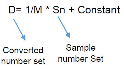
In this case, there is an equivalent conversion (Copt) for the numerical conversion (Cn) that converts the set of sample to the set of converted series equivalent to the equivalent numerical series 1/M * S as follow:

 C(opt) = C (1/M + Constant) * S

To find the series conversion equivalent to the numerical conversion is a question beyond the article.

Tales Conversion in 3D

In 3D our tools in order to find the true conversion C(opt) is more though we have more coefficient in the formula that searches for the C(opt). (maybe in other dimensions like 4D, 5D … our power be even more)

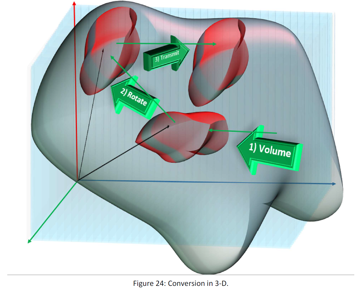
Suppose the following figure: 

Each sample is a vector like (r1, r2, r3) in 3D space. 

There are three coefficients for the conversion in 3D.

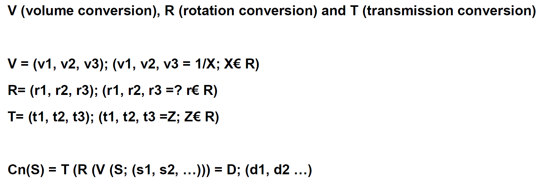
1) Volume: a constant value by order 1/M (M is scalar) multiplies to the sample vectors. 

2) Rotation: The rotation converter makes the vectors rotate and it changes its angular position.

3) transmission: the transmission converter, transmit the vector in the space. 

1) Volume

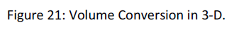
2) Rotation

By means of conversion rotation (R), the sample set will rotate, but the interior characteristics of the sample set remain unspoiled.

3) transmission

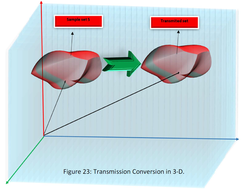
By means of conversion transmission (T), the sample set transmits, but the interior characteristics of the sample set remain unspoiled.

The three conversion is so that the interior characteristics of the sample in them remains unspoiled, that it supposed that the conversion mostly saves the regulations within the data. 

The conversion process in the Tales method is so:

In this way as you see we have three conversions that using them we can find numerous map to the smaller parts of the space. But the true conversion has a condition that the converted set must fit exactly on the points in the space, just like about the 1D space. For illustration suppose that in 2D:

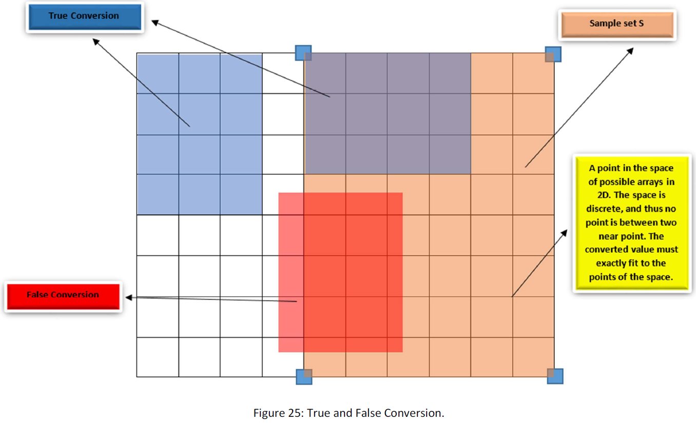
As you see in figure above, the conversions must be so that all the samples after conversion locate on the points of the space, or equivalently the numbers of them must be natural number (N).

Then for 3D space, we have three conversions or Cn (Cn is a conversion that is geometric and works with sample’s numbers, and C is a conversion that works with sample’s series and for each Cn, there is an equivalent C). 

The Cn(opt) is the Cn that satisfies the condition bellow and limit the data is small space as small as possible.

 With this tool, we will have a software that tries for different coefficients in the three conversions and will find one that satisfies the criteria of the compression.

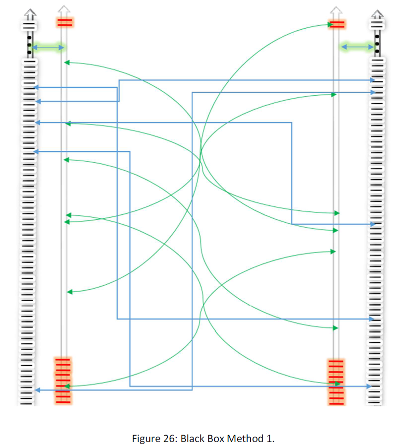
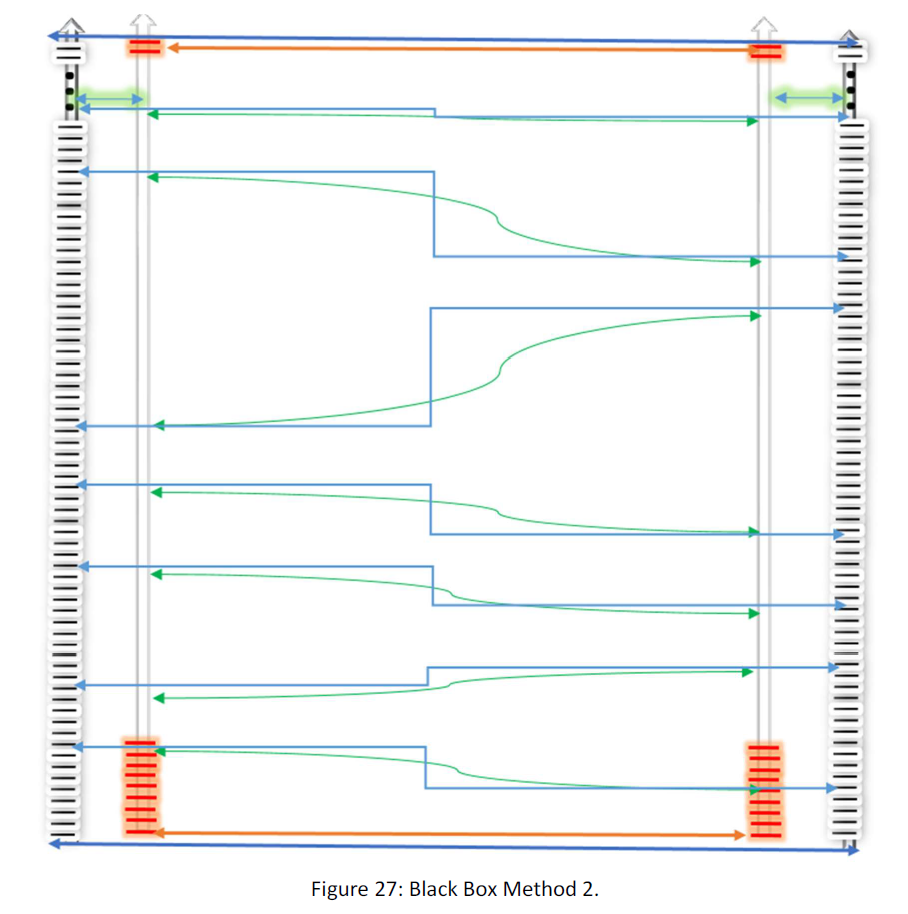
Black Box Method

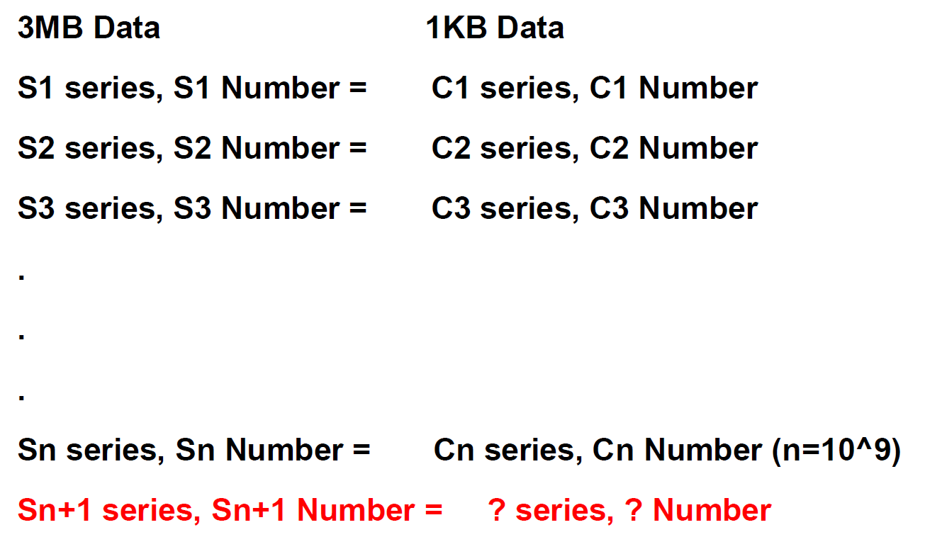
A black box is a software that can learn. Suppose the following:

N1= F1(x)

N2= F2(x)

N3= F3(x)

.

.

.

Nn= Fn(x)

N(n+1) =?

The black box is so that if you give that N1 to Nn value or function or etc., it can guess the next one, or equivalently it can learn the pattern, the order hidden in the given data.

Now I want to use the talent in order to compress data. We have 10 Billion sample data and we presumed a function that map the 10 billion 3MB data into 10 Billion 1KB data as follow:

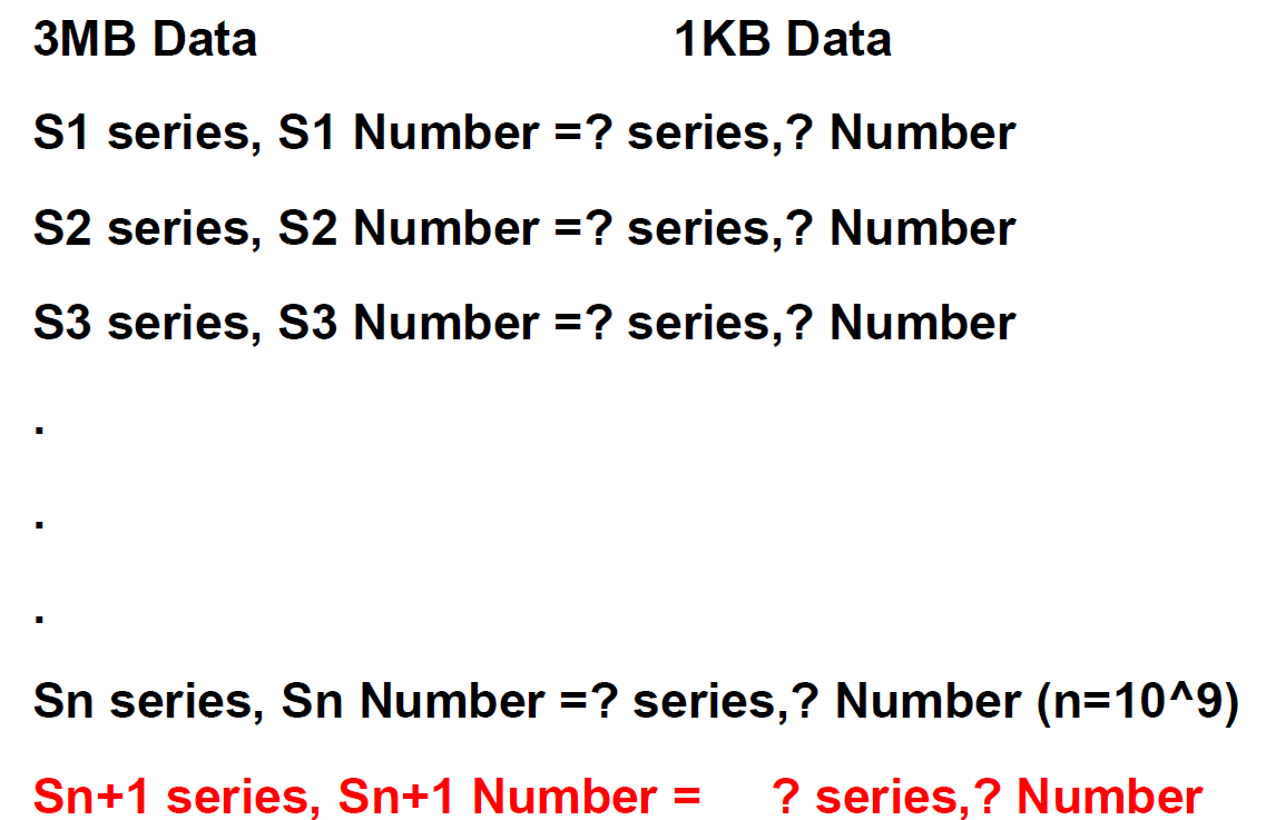
But the point is that in the case of compression, we have no initial data to give to the Black Box. Because for knowing the equivalent of 10 billion 3MB samples in 1KB space, we must know the function and if we know that, then we have the answer and we don’t need the Black Box. I suggest three choices about the situation:

1) Random Distribution

2) A bit information

3) Maximum information

1) Random Distribution

In random distribution we assume that 1) the Black Box is so clever and also 2) there is an infinite or at least numerous map between the space of the kind’s data(3MB) and the small space(1KB). We link the data between the two spaces randomly. Suppose the following figure:

In this case, we gave the other side of the Black Box as follow:

In this case, we hope that the Black Box can distinguish the next Number and Serious. If it happens, we have compressed data, because the function Black Box works with is the function we soak, the one that maps the data space to the limited space. Maybe this needs to give the many random sets of data in 1KB space to the Black Box results and maybe not.

this so unlikely to happen that we get to the conversion in this way. Another way is to give the Black Box a bit more data that it is A bit information method. 

2) A bit information method

In this method, we give only some information to the Black Box hidden in the way we link those random data in 1KB space to the sample data in 3MB space. If we consider the data in 3MB space as numbers and not series, they are numbers that can be ordered decreasingly or increasingly. That each one is previous one plus a number. 

1) We can suppose the order in a way that the data in 1 KB (A’) correspond with a data in 3MB (A) lesser than another data in 3MB (B) is always lesser than the data in 1 KB (B’) correspond with the bigger data in 3MB. That gives a hidden information to the Black Box.

2) The series 0000…000 in 3 MB space Correspond with the series 000…00 in 1 KB space and they are Zero. And The series 1111…111 in 3 MB space Correspond with the series 111…11 in 1 KB space and they are One.

The two boundary conditions are depicted in the figure below:

By this information may be the Black Box be able to discern the regularity or order between the two space or make it. 

In the third method, we even give more information to the Black Box hopping that it can discern the true conversion or C(opt).

3) Maximum information

In maximum information method, we try to give the Black Box as more information as possible. In addition to the data we gave it in a bit information method, we give it a bit more. For this purpose, we need some features that can be numbered in the sample data in 3MB space. Characteristics like the repetition of a code, the number that the samples number can be divided into two or any other numerical characteristics, those could be found in number theory. Suppose that we have five characteristics that each one can be numbered.

The characteristics can be named as: 

{U1, U2, U3, U4, U5}

Now we want to distribute the ten billion samples in the 1 KB data space considering the characteristics. Let’s multiply the characteristics into each other. 

U1*U2*U3*U4*U5 = P 

The number of 1 KB set members is 2^8000. the number we allocate to each sample must be a multiple of P. in this way, the characteristics somehow included in the way the 1 KB random samples distributes, and we can hope that the Black Box discern the order.

Using the Cullatz Puzzle in the Black Box

There is a puzzle in mathematics that tells any number within the function:

Even: * ½

Odd: *3/2+1/2

Will ends to one. It is not proven, but also all attempts to deny it has failed. We can use the fact to give the Black Box good distribution in 1KB.

Suppose that we put all ten billion samples into the function. The function decreases the number to one. But there is a point that for each sample, the number becomes less than 2^8000 that is a number equivalent to a series in 1KB. The point is the equivalent series in 1KB for the series in 3MB. (the possibility that two sample’s series pass by one number less than 2^8000 in the first step to space through to the greatness of the numbers is so few and approximately zero.)

Then we give those series in 1KB to the Black Box as the equivalences of the samples correspond data in 1 KB space.

4) samples box from 3MB samples

Suppose a 3 MB series. That would be something like this:

We want to sample 1 KB from the 3 MB, that is equal to 8000 zero and one or boxes. There are many ways to choose the 8000 boxes. I try it in the most regular way. Divide the 24 million to 8000.

24*10^6/ 8* 10^3 = 3* 10^3.

Then choose the first box of each 3000 box (or last box). In this way, we have a 1 KB data equivalent to the 3 MB data. We name the data T(S).

We have 10 billion 3 MB samples. Thus we have 10 Billion T(S). We gave the T(S) to the Black Box. (Again because of the greatness of the numbers, the possibility that two samples have the same T(S) is approximately Zero.)

Then we have:

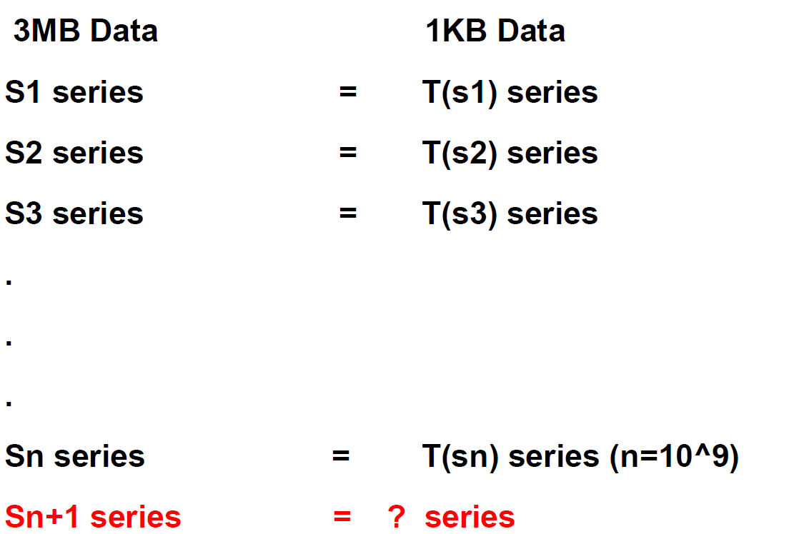
It is possible that the Black Box can discern a regularity by the information given to it as T(S). Because T(S) is somehow like the heart of the sample. 

Two Other Methods

1) Cullatz Puzzle Method   2) Geometric Method

1) Cullatz Puzzle Method

Suppose the puzzle I told above. All numbers will end to 1 by the function. The function is:

Even: * ½

Odd: *3/2+1/2

We put a number into the function. We put a number into the function. There will be so;

EEOEOEEEOEEO…

Even is 1 and Odd is 0. For any number there is a series that leads to 1, thus there is an individual series for each number that can be shown as follow:

110101110110…

Point: 

 the possibility that the function is even is more, because after an O or 0 inevitably the function is E or 1, but after E or 1 there can be still 1. Thus the series is capable to be summarized. 

This function is so that for some numbers the series becomes so huge, and for some other, the series is so short. For instance, for number 7, the series goes high to 1000 and backs, but for 1024, immediately it goes to 1.  As if for some of them the series is so small and for some huge and this has no order. A number turns soon to 1 and the next number series is so huge. Though we can use this fact. Suppose the following figure:

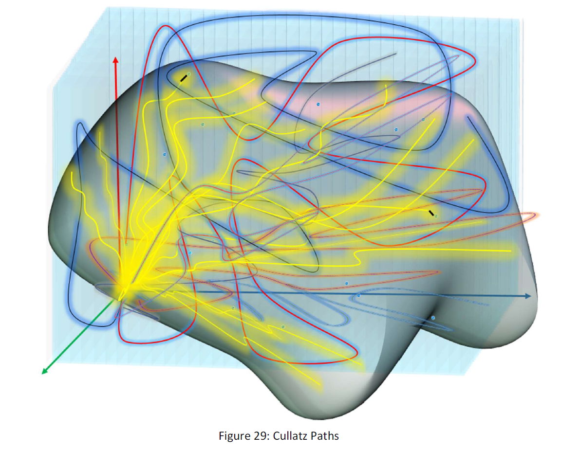
 Each line is the points that the if we put the end of the line point value in the function, it passes through the point that is covered by the line. And for each point, there is a line and for each line, there is a unique P function series shows the order of use of the functions (E) and (O). In 3D each point is three 1 MB series and number and for each point, we have 3 series. The Golden lines are those series that reach to 1 in a short pass and equivalently series. The lines are other colors are those their P series is long and thus not efficient for our purpose. 

First I claim that maybe the P series of any point or equivalently any data in 3D space, be used in many kinds of compression. Because though the reason I said previously, the repetition of E function or 1 is more probable and thus may we can find some less heavy literature to represent the P series. But generally, no literature compresses all the 3 MB and if it compresses part of the data space, for instance, 30%, it increases the rest of space volume 70%. But I just suggest that maybe the literature P function or equivalent P series of the data be helpful in compressing data.

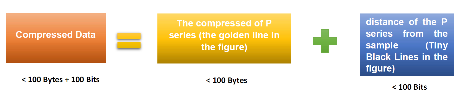
My Claim About the Use of P series in Data Compression

Point 1: For each point in the 3D space of data there is a unique P (p1, p2, p3) series. 

Point 2: In each tiny part of the space, that can be addressed from within the space with so tiny amount of data (for instance, 100 bit), there is a P series that reach to one so fast.

Thus the P series is short and also for that the repetition of the E function or 1 is so much, it can be abbreviated or equivalently compressed in a so high degree. (in the figure the series belongs to the golden lines that spread all the space.)

For instance, a golden P series will be so:

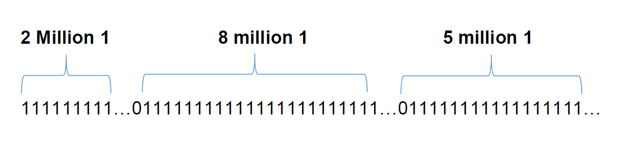
Then the series can be compressed in a tiny space, for instance, 100 bites.

Hopping Result

We hope that by this method we can compress data in a so high magnitude as follow:

Geometric Method

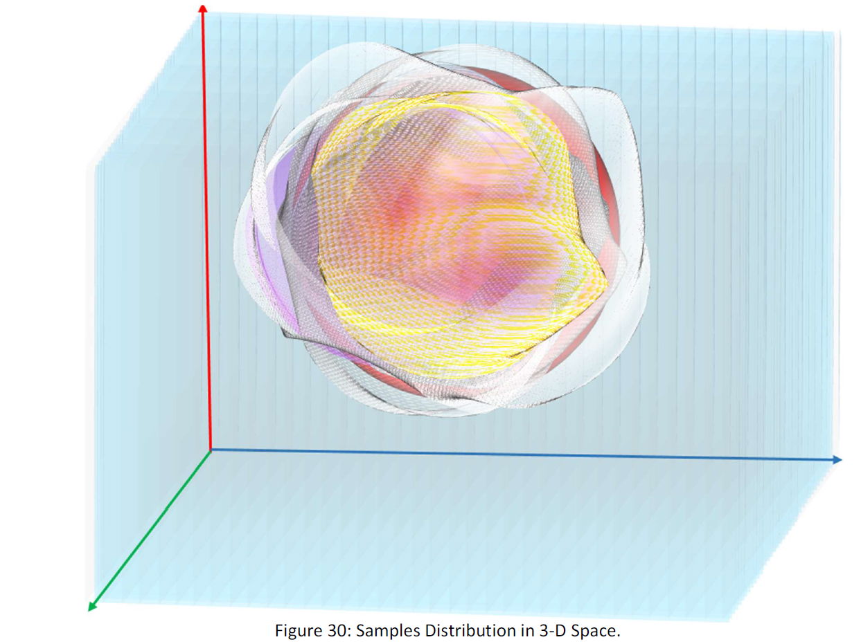
Suppose a kind of data that each member of that is 3MB like a movie frame. Every 100 Bytes of a 3 MB data is a number and each 300 Byte is a point in a 3D space. Then the 3 MB data is 10.000 point or equivalently a 3D shape. 

Now suppose those 10.000.000.000 samples. They are 10.000.000.000 3D shapes or more precisely, 10.000.000.000 distribution of the points. r

The idea of the Geometric Method is to find the average shape of the samples, and then address the new data from the average shape. 

Suppose the following figure:

In the following figure, the red sphere is the average of the shapes (the shape obtained through evaluation and I chose sphere for ease of illustration). We give that to all the receivers and just send them the deviation from that in each data. 

Suppose the following figure:

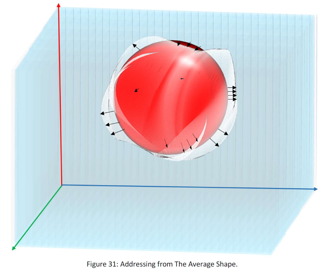
Still, we have 10.000 points, but the points can be addressed with less than 3 MB. Each point is represented with 300 Bytes. Suppose that with that with the method we can reduce that to 1 Byte. If so, we are able to compress data to 1/300. 

We said that we give the receivers the sphere (any shape) that is 3 MB as a default value.

Then we just send to them the deviation value (D). Then or data contains 10.000 of 1 Byte deviation value. This is 10 KB. This 10 KB must be converted to the main data in the receiver as:

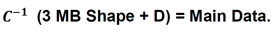
At this point, we can use the other methods with the 10 KB deviation series. For instance, we can use the Tales Conversion Method, AI Method, Cullatz Conjecture Method or any other method to compress the data more.

Point 1:

as more capacity we deduce for a point (in above 300 Byte) we can search for more powerful compression, but we lose precision. Suppose that for each point we deduced only 3 Byte, then if at must we were able to reduce the amount to 3 Bit by the method, we would compress to 1/8. We can compensate for the matter of precision by increasing the data samples.

Point 2:

We can imply conversions on the all 10.000.000.000 samples, in order to find the conversion that makes the samples most near to each other, thus this would need the least amount of data to record the deviation from the average shape, and thus consequently least amount of data to address to the data.

Point 3:

There can be points that are in common in all the 10.000.000.000 samples. We can assume that they are common in all data in that Kind. We investigate that in the next Method I call it Bolter Method.

Bolter Method

In bolter method we put the 10.000.000.000 samples under each other as follow:

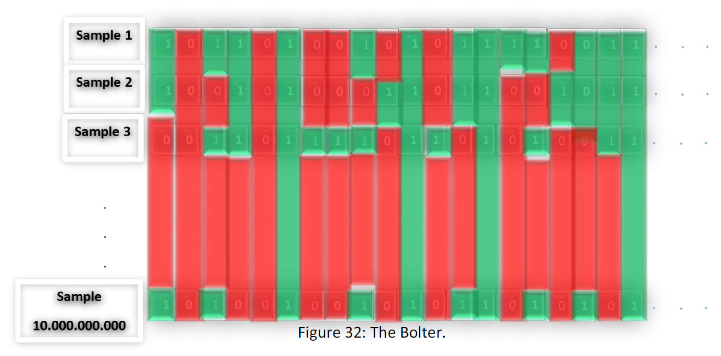
As you see in the above figure, the bolter makes the box with value 1 green and the box with value 0 red. In this way the boxes that in all the samples are 1 and 0 becomes completely green and red, and the name bolter is because of this, because in the cases, the system behaves like a bolter, and the remained boxes with value 1 and 0, that have the same value in all the 10.000.000.000 samples are the characteristics of the data kind. 

Also, the bolter gives a percent of occupancy of 1 and 0 in all boxes. At the end the bolter's output is something as below:

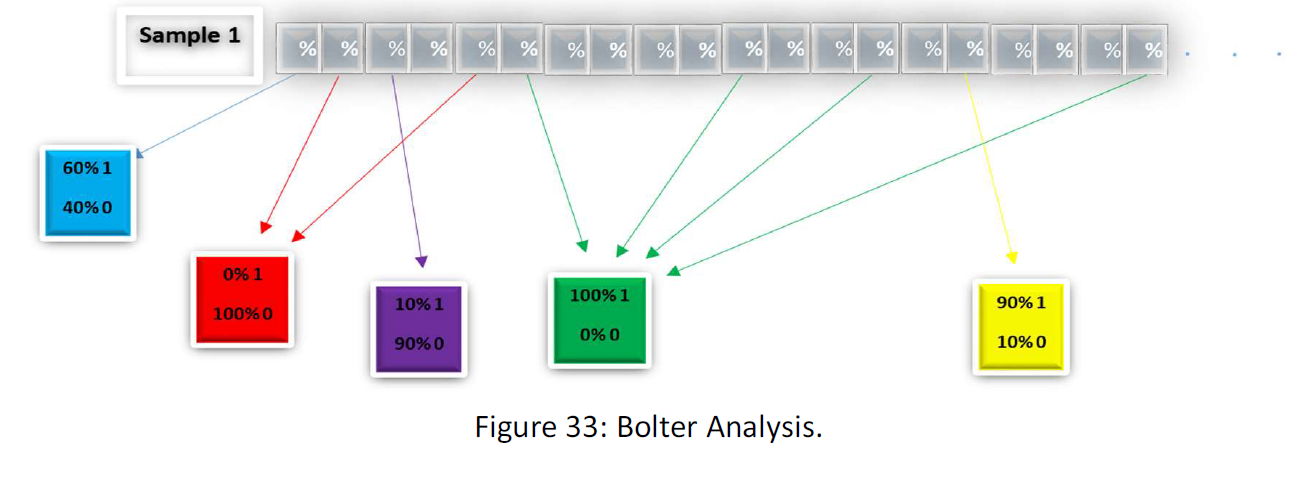
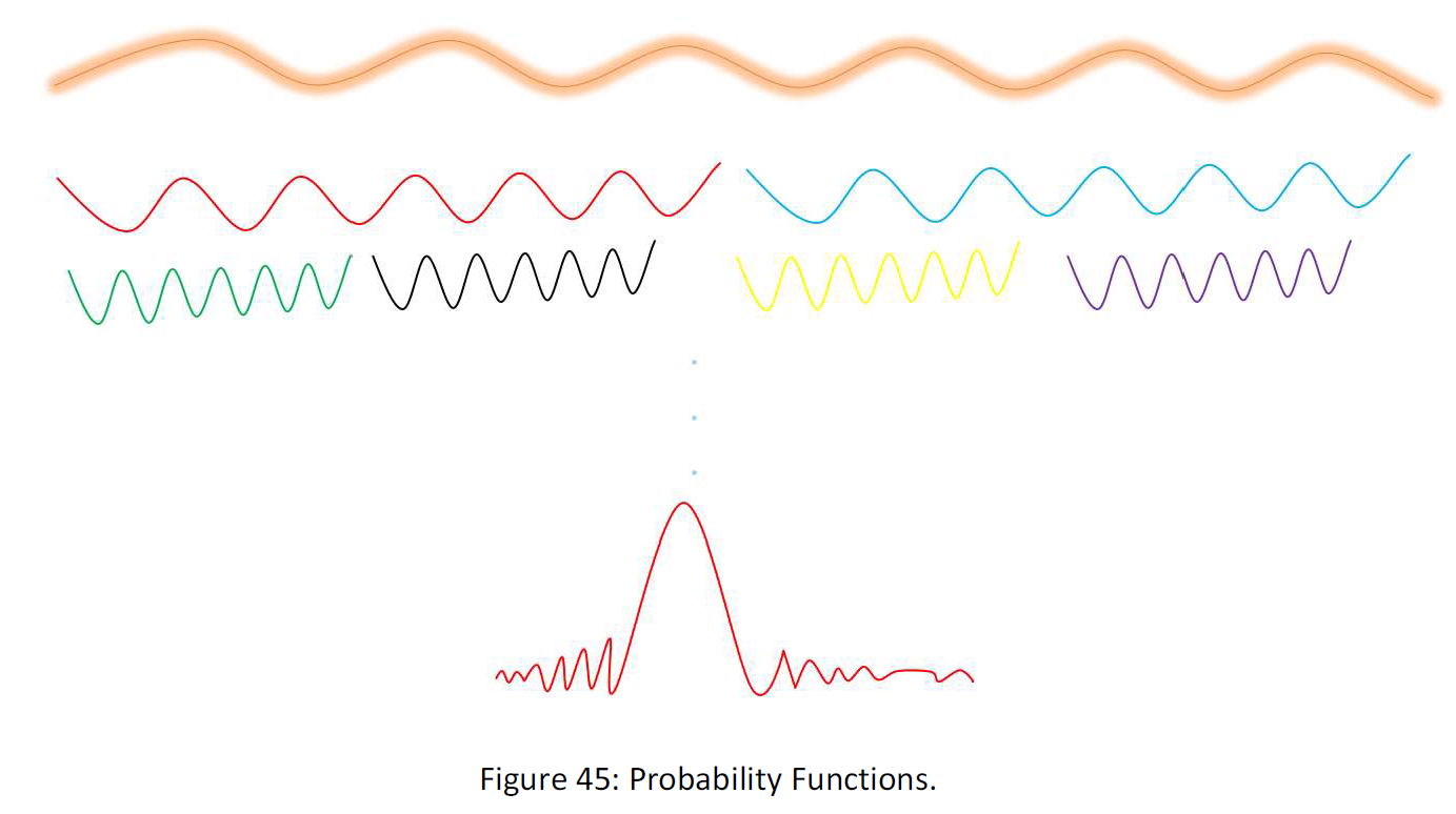
In this way, for each Box, the bolter gives us a pair of percent for 1 and 0 in all the 10.000.000.000 samples. And that would be a function as the following figure:

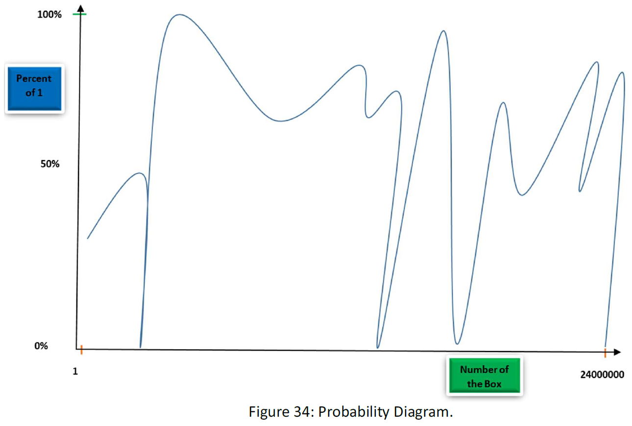
That would be a shape like the above figure that for each box gives the percent of the boxes in 10.000.000.000 samples with value 1. The function of the percentage of 0 in each box can be obtained by the function and is in that.

The percent of value 1 in each box is the probability that the box has value 1. In this way, we can calculate the possibility that for instance, the boxes 1,3,5,7,16,18,20 at the same be one. Suppose that each one has the possibility of 60% to has value 1. Then the possibility that they are all 1 is (60%)^7 = 0.027994. In this way, we can calculate the possibility of each data in the 3MB space. Each data is a set of 1 and 0 with a possibility in a 3MB space. Then the possibility of the occurrence of the data is the possibility of each box with that value that is a multiplication of 24 million possibilities that, of course, is a very small value. 

The purpose is to evaluate each possible 3MB data possibility and if we can do it, we have done. Because in the case, we know that where in the space of possible arrays in 3MB, the data has concentrated. 

Question: But how to evaluate that?

1- Evaluation One-by-One

The way evaluation is to calculate each possible array in 3 MB and then get to the distribution of the possibility of the data in the space. This way somehow seems impossible. Because our computation power is not infinite, at least now.

We have 2^24000000 possible arrays and each array possibility is a multiplication of 24000000 numbers (Possibility of their box value). Then to obtain the distribution of the possibility in this way means to calculate and categorize 24000000*2^24000000 multiplication that seems impossible. 

2- Algebraic Method

In the algebraic method, we seek an algebraic relation between the two space. (the space of 1 and 0 possibilities in each box and space of distribution of possibility of possible arrays in the space.) There can be a function as follow:

G = the space of 1 and 0 possibility

H = space of distribution of possibility of possible arrays in the space

F(G) = H

But how to find the function F?

I suggest a way to find the function, but first, let’s consider what kind of function could be the H. Suppose that all possible arrays have the same possibility to happen. This is for the case that we have no sample data and all the possible array has the same possibility to happen. Suppose the following figure:

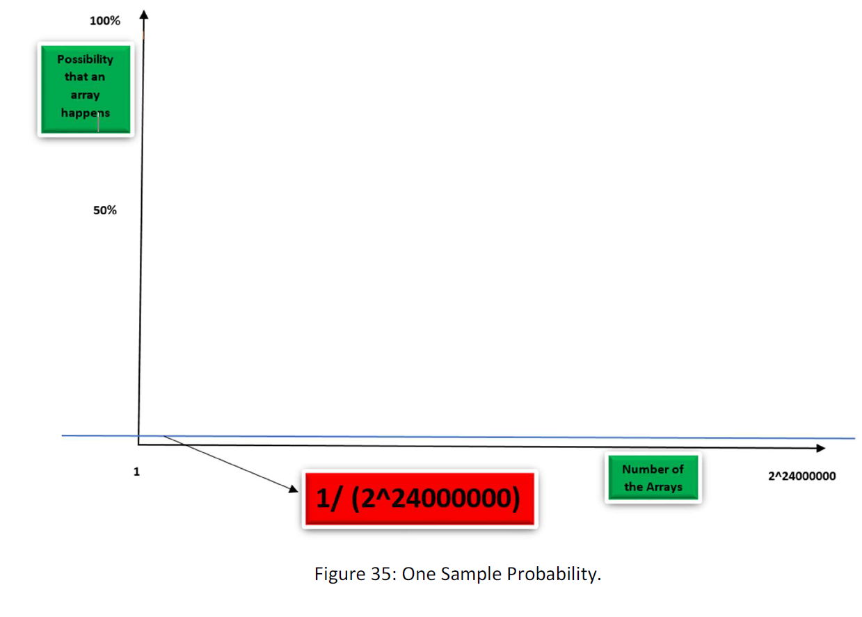
There is no sample, thus all arrays have the same possibility to happen. Though there are 2^24000000 possible arrays in 3 MB, then the possibility of each one to happen is

½^24000000

Now suppose that we put one sample into space. Suppose the following figure:

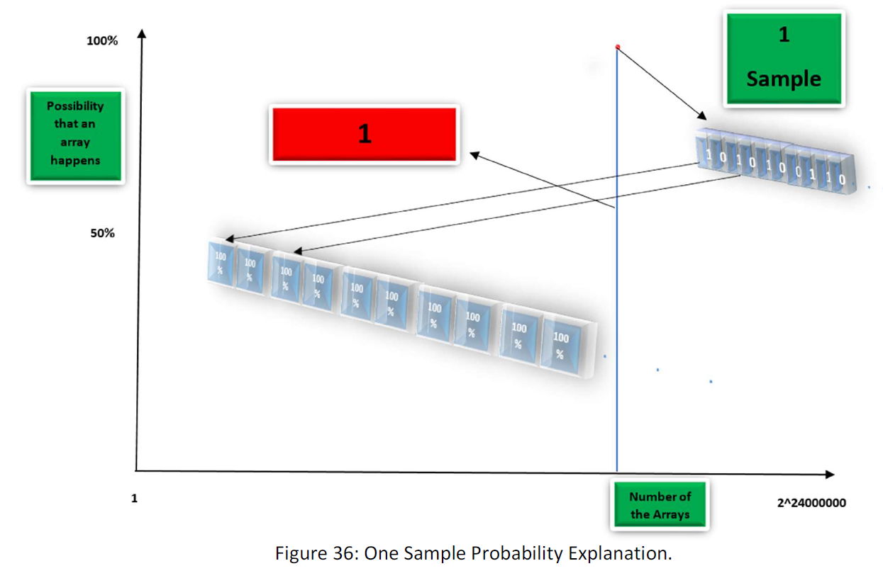
Though there is only one sample, the probability of 1 and 0 in all the Boxes is 100%, and consequently, the probability of the occurrence of the array (as this is only this) is 100%.

Now suppose that another sample is input in the space. Half the sample’s 1 and 0 differs with the first sample as follow:

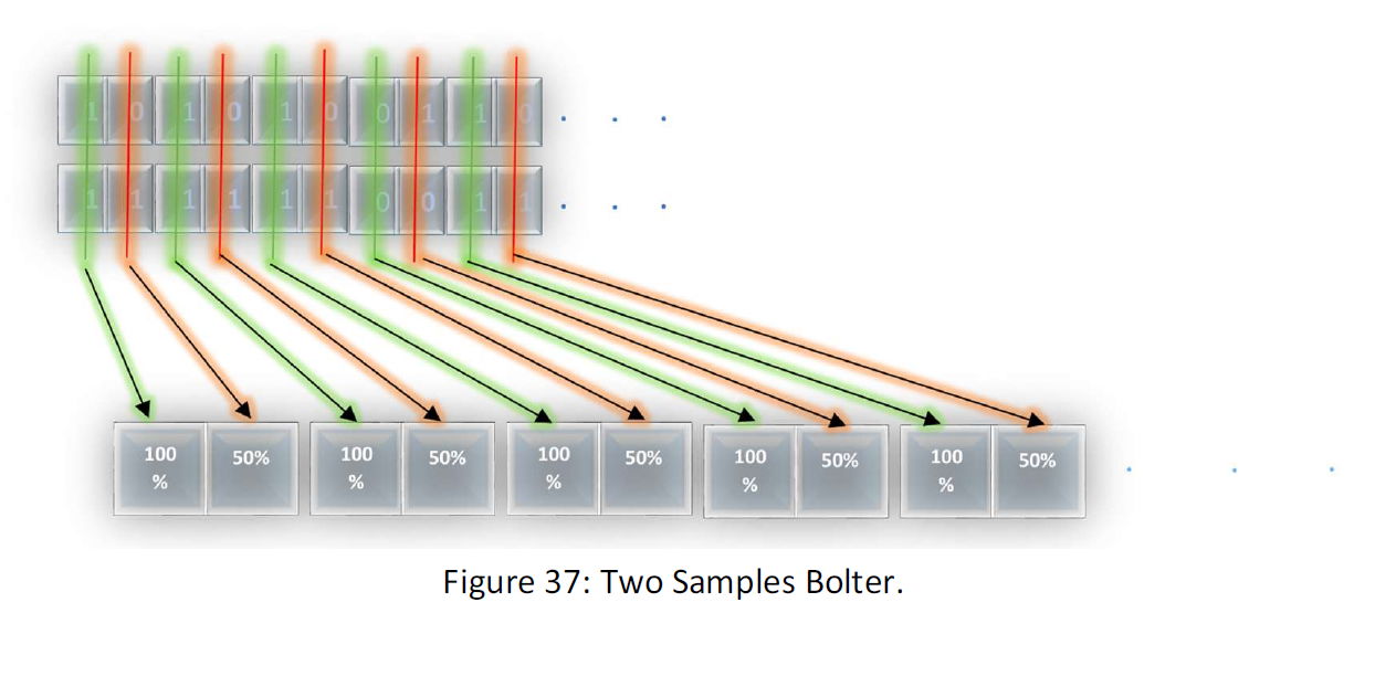
As you see, the second sample changed the distribution of probability of 1 and 0 in the space. With the new distribution of the probability, we will have a probability of ½^12000000 for the 2^12000000 possible arrays. (you can calculate that, there are 12 million Boxes with determined value of 1 or 0 with a probability of 100%, and 12000000 Boxes with a probability of 50% for 1 or 0 for each box) 

The distribution of probability will be so:

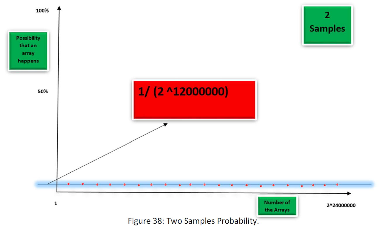
We have 2^12000000 possible arrays and each array with the possibility of ½^ (12000000). Now suppose that we increase the number of samples. 1000, 1000000 to 10000000000 samples. Gradually the distribution of probability will changes as follow. 

Suppose the following figure:

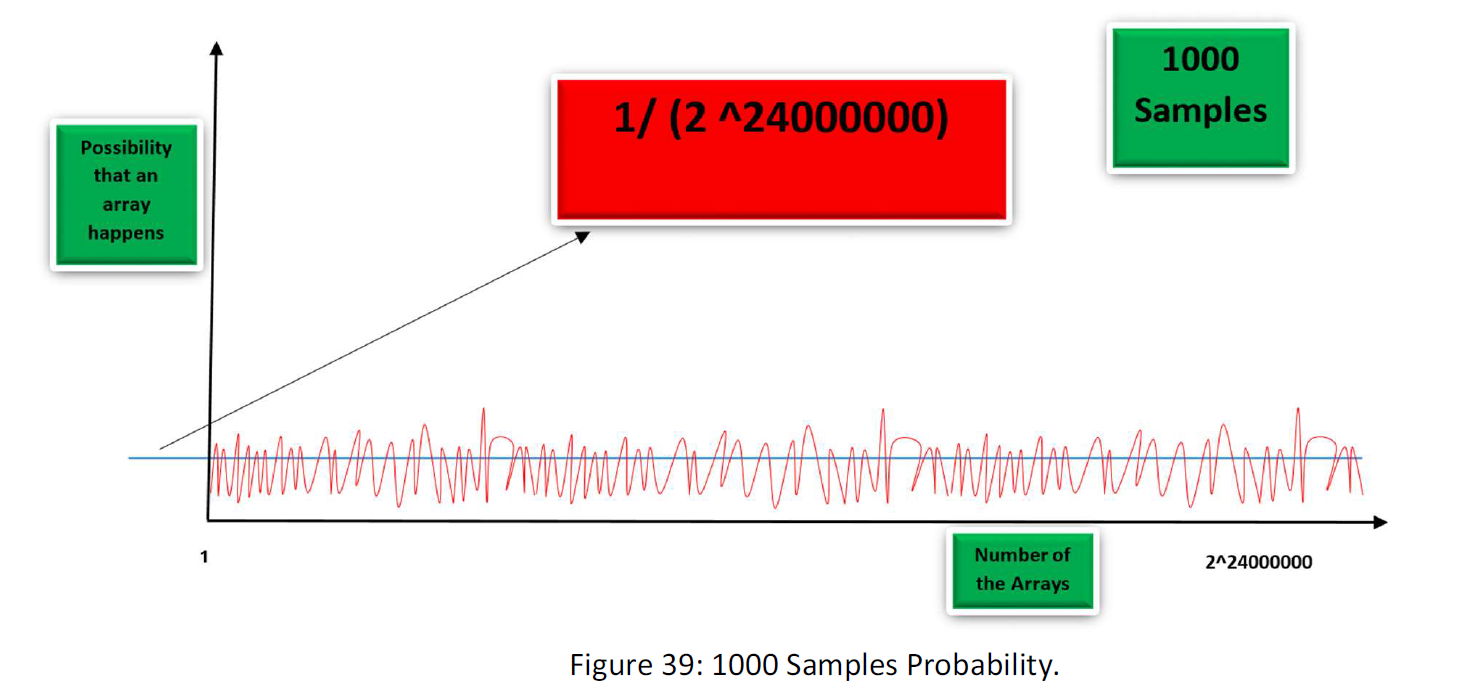
Adding More samples, we will Have:

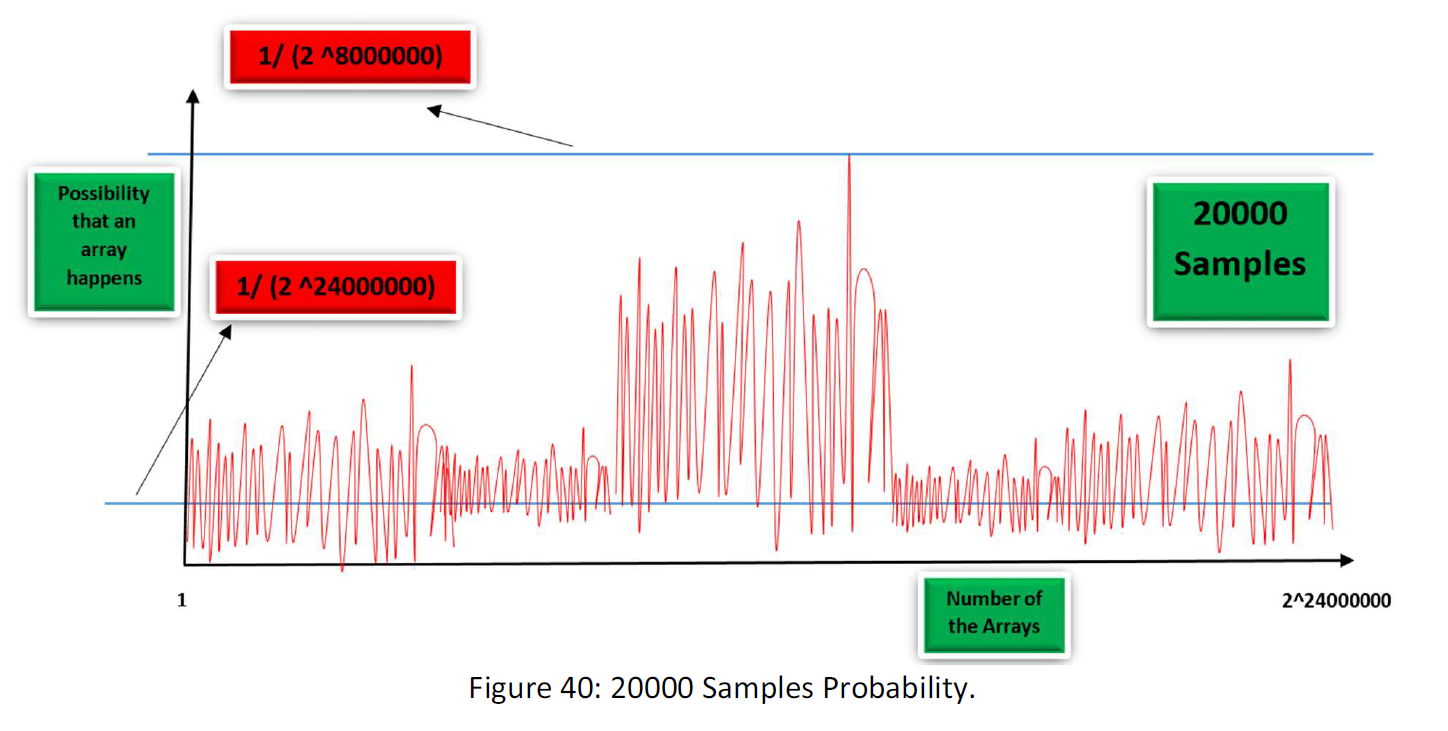
Adding More Samples, we will Have:

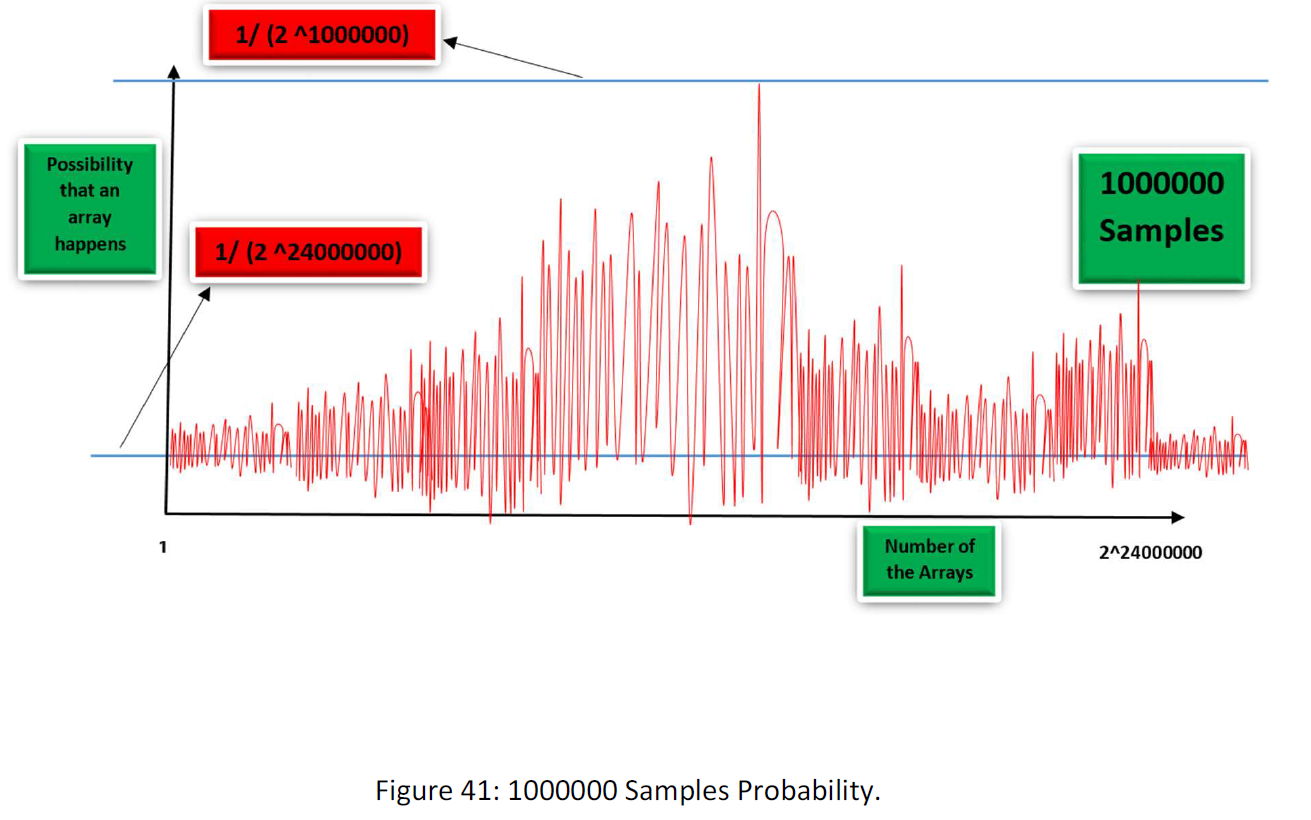
At the end for 10000000000 samples maybe we have a diagram like this:

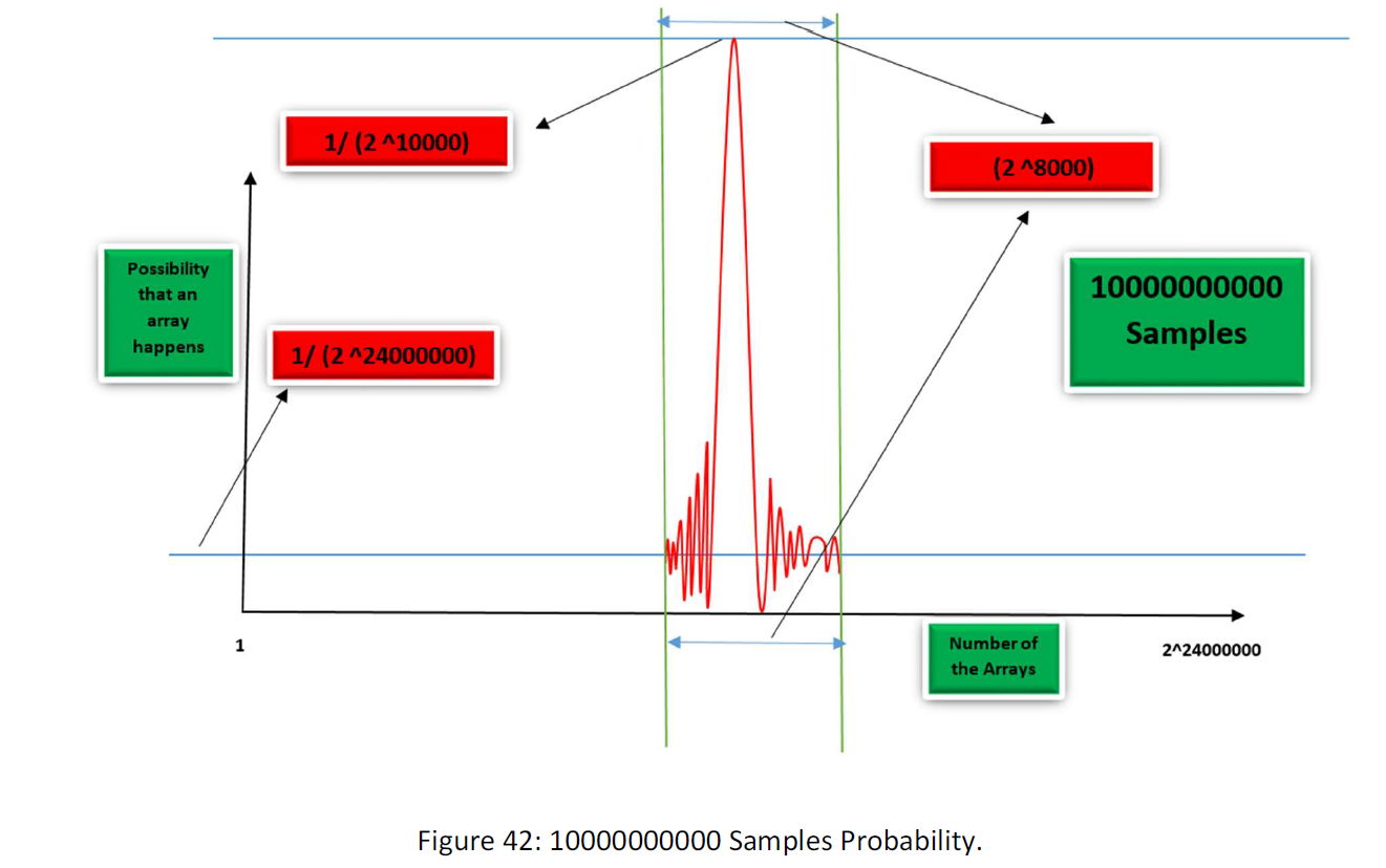
As you see gradually as more information fed to space, the function collapse within a tiny fraction of the space. Space is like a planet within the vast space of the data that our data kind nest in. Of course, this is my guess and I just wanted to explain the procedure. Maybe there be some planets and worst, maybe at the end, we meet chaos and not an order. 

I claim that there would be an order for two reasons:

1- The data have featured in common.

2- The number of data is so few rather than the volume of the space.

The first reason says that there is a hidden regularity that increasing the samples, leads the function to the last one. That more samples we have, we are able to predict the next sample more precise. That’s just like nature. As more data we receive, by true evaluation and analyze, thee is able to predict it more exact. 

The second reason is more controversial. There is a question.

 “Does any set of samples hide a regularity inside themselves?” 

I think the question more than scientific is philosophical. By a realistic principle, I think No.

There must be an order within the data that be distinguishable. But I told that as a reason because we have a real regularity and also the numbers of samples are few, thus there is a way to limit the data kind within part of the space, the tiny part.

I think this is the matter of truly defining the space and conversions. That the way we define the space, (that which series is 1, and which series is 2 etc.)  and if we chose a space, the true conversion that makes the data limited in part of the space. They are one, whether you take time to find the convenient space or true conversion. Or maybe the combination of them is the way to find the true compression. To set a true space and seek the best conversion within that. (Like a physician that based on a true theory tries to solve a problem. The theory is the space, and to solve the problem is to find the true conversion. That I said with a realistic principle, I found the subject as a philosophical one. This is like trying to make Chaos ordered. Like what we do in philosophy, science or religion. A true language structure, a scientific theory, or a belief; they are ways to discern or find order in the Chaos. That I said realistic principle, I meant that there must be an order inside the chaos that we can find it. If there is no order inside that, we can’t find any. That the order we find as a scientific theory exists there in nature, and that is not so that the scientific theory is just inside our minds. It has an equivalent out there inside nature. The order we find here is just the one exists in the data, even as the belief of a director, or the way people think or the way the codes are arranged when they learned them to the cameras and receivers. They are there and we just unveil them, and if the orders don’t exist, I think we cannot find them or imply them to the data. This is both mathematical and philosophical question. Mathematical because we can calculate the possibility that a random set of data has an order (of course after defining order mathematically), and philosophical because this is the matter of reality.) 

A way to obtain the probability of distribution of data

Suppose that for 10 billion samples we have such a probability for each box:

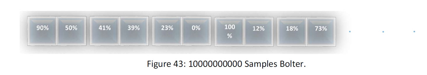
That is a 3 million numbered series like this:

(90,50,41,39,23,0,100,12,18, 73…)

And the series is the probability of 1 in the boxes. There is an equivalent series for the samples for the probability of 0 in the boxes as the same, as following:

(10,50,59,61,77,100,0,88,82, 27…)

Then for a set of samples, we have the probability of distribution of 0 and 1 as above.

You can consider that as two functions also. Now we consider each two box as a box as follow: 

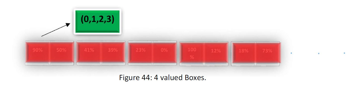
Each box can contain four-value (0,1,2,3). The four value is the probable arrangement of 0 and 1 the could have. Now for the new composition, for each set of samples, we have four series or functions for the probability of each value. 

Series (0): Probability of 0 in each box.  Series (1): Probability of 1 in each box.

Series (2): Probability of 2 in each box.  Series (3): the probability of 3 in each box. 

we also consider each 3 box as a box. The box will have 2^3 or 8 possible value. Then we will have 8 series or function. For the box of 4 boxes, we have 16 series or function and etc. 

In the process, the last step is to consider all 3 MB or 24000000 boxes as a box. And the probability of each possible number or array is what we want. 

Of course, to do all the steps takes so much computation and thus, time. But maybe there is a detour. Suppose the following figure:

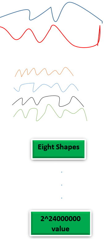
3 million boxes of two value 0 and 1:  

(2 of 3 million numbered series)

1.5 million Boxes of four value 0 and 1 and 2 and 3:   

(4 of 1.5 million numbered series)

1 million Boxes of 8 value 0,1,2,3,4,5,6,7: 

(8 of 1 million numbered series)

1 Boxes of 2^24000000 values 0,1,2,3,4,5,6,7,8,9, …

(2^24000000 of 1 numbered series or number) 

As you see as we go forward in the process, the number of series or functions increase, but the number of each series or length of the function decrease, and at last the length of the function becomes one, and that is what we want. This is like the following figure:

And at the end, there are 2^24000000 points or numbers. (each two function are equivalent like function for 0 and 1 that can be obtained by each other.)

We can inductively find the way the functions are converting in each step. For instance, we can find functions for 2 numbered, 4 numbered, 8 numbered, 16 numbered, 32 numbered 64 numbered and 128 numbered boxes. Then we can guess the way they are altering in each step and consequently, we can obtain the conversion between different phases. If so, we can obtain from the 0 and 1 probability series, the function of the probability of each possible array, (the last function), and that is what we want.

Irrational Numbers Method

The last method is the one I thought of first when thinking about compressing data, that I thought better to include that in the article. Actually, the thought that led me toward the subject was not about the computer, but a philosophical question. I watched Morgan Freeman documentary. A philosophy teacher in the documentary claimed that “we live inside a computer.” I was thinking about an answer to his claim. I told myself, “what if the data of the world be infinite, then how it can be inside a computer?” 

Then I forget the professors claim. Just suppose that you can measure a bar by infinite precision. Whole your life you can try to measure it and add another fraction to the length.

(forget the quantum mechanics.) then I thought, if so, how an infinite world can be represented finitely or understood? Then I remembered the notion of irrational numbers. They are like pairs for rational numbers. Suppose Radical 2. In rational representation that’s an infinite serious that is not periodical. I thought maybe the world is also so. An infinite rational with some finite irrational. In this way, irrational numbers are not numbers, but like machinery that produce series. Suppose that the world has an irrational part that is producing the rational part. This is deterministic, but those numbers are both there and are not until we find them. Anyway, I thought that leave the philosophy, how it can be used, that I thought of computer and data. That’s a dream, if instead of a DVD, we give the client a Number, and tell him, “Count the Radical of the number by yourself and enjoy the movie.” But soon I get that that is impossible fundamentally. Because at the end for sending the radical, the message, we need to send it in binary. And if we want to send 1GB in binary through 1 KB, there must be a One-to-One map between the 1 GB and 1 KB space, and we know that there is no such thing. That is a data capacity reduces in radical literature, the other one increases. 

Then I thought of so great are the possible arrays within 1GB or even 1KB. What if to find a part of 1GB that we work with. That I reached to the article idea. 

But now I think we can use radical numbers. Suppose that within the space that our data are limited in, we can find an equivalent series of a radical series. And maybe we can find many. The radical series can be dots in the space that we address by them. They are like the countries name in addressing a house. Country of radical 2, radical 5 etc. I suggest that maybe they can be used.

The conclusion to Compression Methods

Four main approaches have been suggested to compress data. Maybe they work individually or maybe the true way is to combine the methods in order to reach a way to compress data. The method Tales and the method Bolter in two distinct way try to limit an area that the data are trapped in. Maybe the two can be mixed with the method Artificial Intelligence. The method puzzle and radical also are ways to summarize addressing. Maybe the five methods together can get us to a better compression, and may be individually they work.

Order and Compression

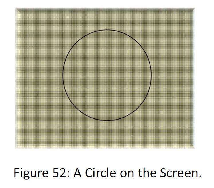
As if there is a link between the two notions “Order” and “Compression” . Suppose that you have a screen that can have two values, white and dark. This screen can depict many shapes. Now Suppose that the screens have 2^24000000 points, that means for coordinating the point of the screen there is 3 MB data needed. Now suppose that we want to send a shape of a circle from the screen to a receiver by data. We have two ways. Suppose the following figure:

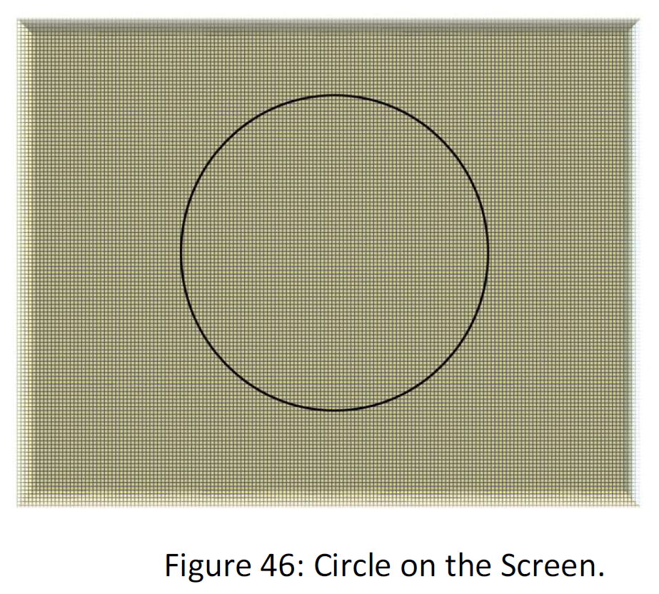
There are two ways to send the data

1) by sending data of the screen. That is 3 MB 1 and 0 for characteristics of the cells.

2) to send the regulatory that, all the points that are from distance R from the center A. (The discrete of the space may cause a trouble for the defining the circle in this way, but that’s just for illustration.)

Suppose the following figure:

As I said there are two ways to send the shape:

1) By data: that’s a 3 MB data

2) By the command that: all the points that are from distance R from the center A.

Then there are two ways to send the data. A direct one and an indirect one as follow:

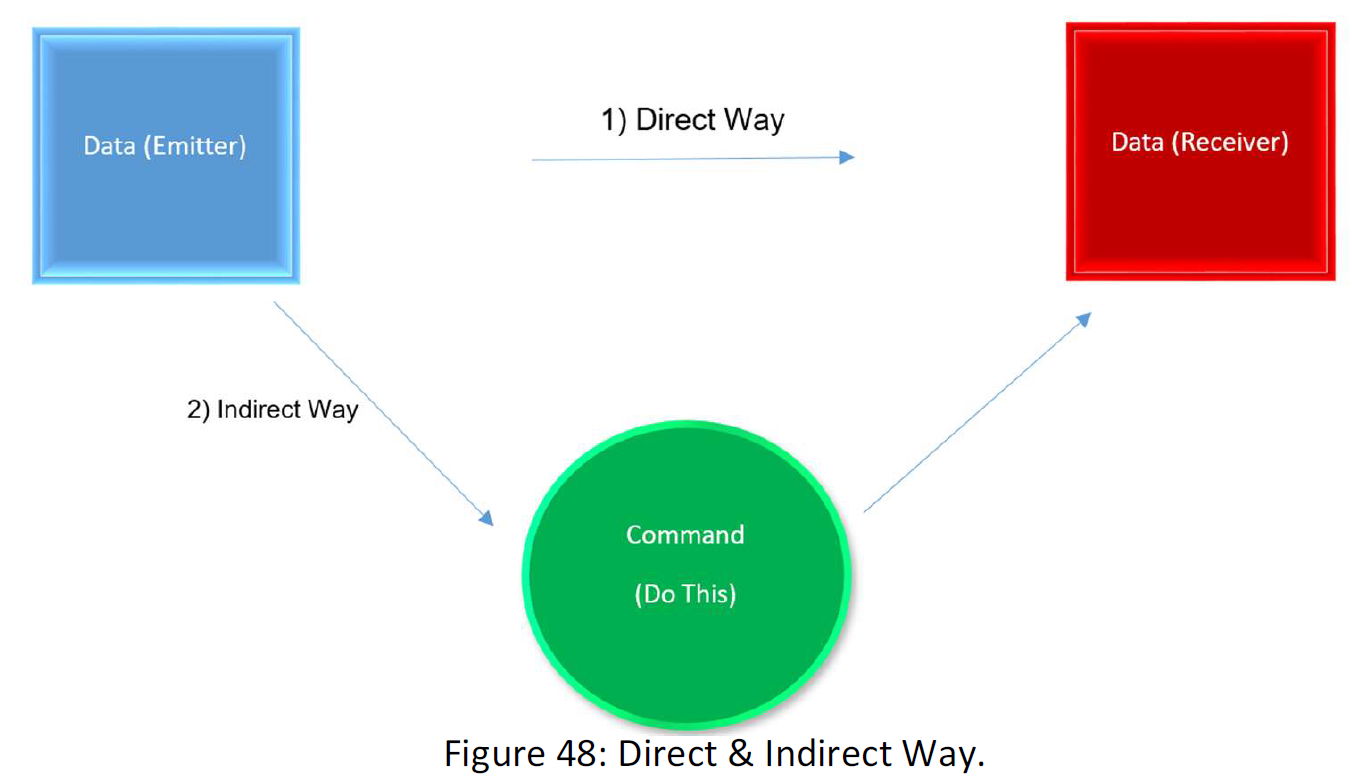
The compression process is to send data through a command or a set of commands. For instance, in the above example, the command is “light the points at distance R from point A”. But at the end, the command is a code contained 1 and 0. If there ought to data be sent through a command, all the 3MB possible arrays that are 2^24000000 must have a One-to-One equivalent in the language of the command. If not One-to-One, the receiver cannot appoint the command to the right data, and one command can refer to two data.  Suppose the following figure:

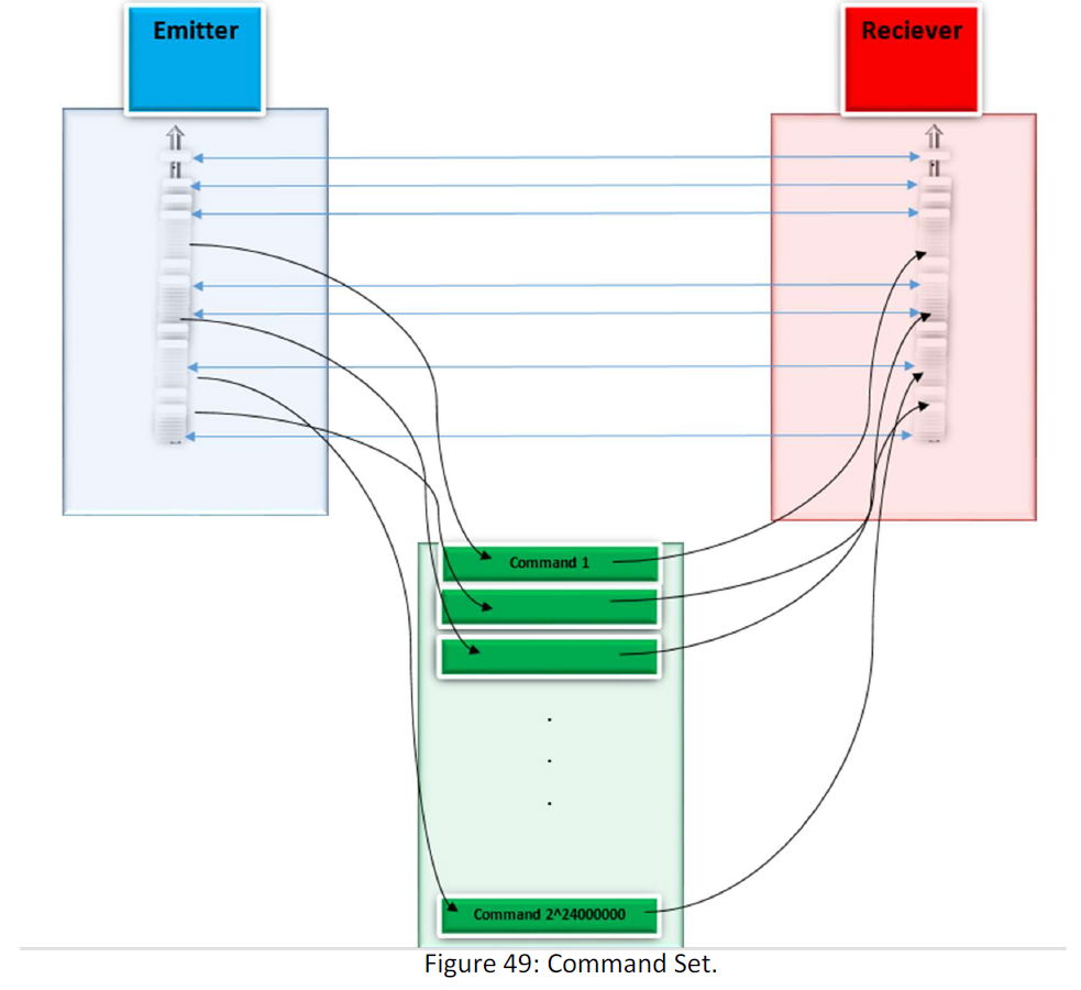
We have 2^24000000 distinct data, and if we want to send them through a literature(command) for each possible array we need a distinct command. Then for 3 MB data with 2^24000000 possible arrays, we need 2^24000000 commands. 

In the end, the commands also have equivalent in binary as 1 and 0. Then there is so:

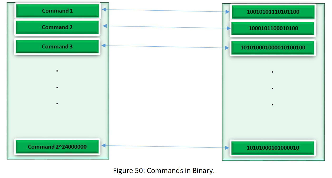
For each command, there is a set of 1 and 0 in binary. We have 2^24000000 commands, then the space that can contain 2^24000000 commands at least must contain 2^24000000 points that is 3 MB space.

Now what we do when we compress data? 

The space of the commands in binary has the same numbers of sets of 1 and 0 as the space of the 3 MB data. Look at the data as number not series. Suppose the following figure:

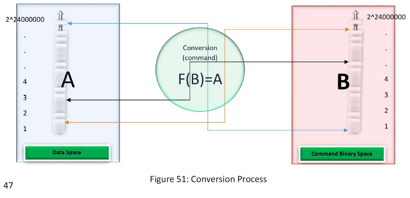
In this way, the function converts binary data to the command binary data. When we compress data, the data as if works so:

F (235) =2^23000000+ 900234345034553

The receiver knows the data and in this way, we compress data, by means of representing a big number with a small number. But there is a point.

when a command set to map a big number to a small number, also it maps a small number to a big number, and this is inevitable.

The important above point is what I meant by this part of the article. In ordinary sending the data, 1=1, 2=2, 3=3 …

But when we use compression, we use a function and as if there is:

1=F (2^23000000), 2=F (2^12000000) ….

But in this way, as each number in the data space links to a number in the command space, when a small number links to a big number, a big number links to a small number and this is inevitable.

Let’s back to the first example. Suppose that screen:

Suppose that we send the data above with a command:

“all the points that are from distance R from the center A.”

Suppose that instead of 3 MB, the command occupies less than 100 bit, but another data will occupy more than the space it occupies in the ordinary way of sending data (not by command). For instance, for the one point below may be in the command literature, you must spend 3 MB space.

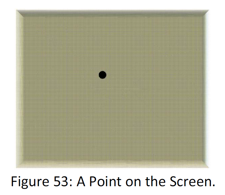
What is Order?

“Based on a command set, when we are able to compress a data, we say that the data has ordered.”

Point 1: Order always accompanies with the disorder.

Point2: There is no command set that can make all possible data ordered(compressed).

Let me explain the above definition. Suppose the 3 MB screen. If we want to compress the circle we say: “all the points that are from distance R from the center A.” 

There is a geometric set of commands that convert those points data to this command. But the point is that, if the command set reduces the capacity of data of the circle, it increases another shapes volume. 

When the volume of a data in a command set decreases we say the data has order based on the command set.

Also when the volume of a data in a command set increases we say the data has  disorder based on the command set.

That’s the Data Space. Now we want to translate the data space to the commands based on a command set. This is like to look at the space with the glasses of the command (like a theory). As we said, the number of commands is equal to a number of the points of the space. Some different conditions may we meet as follow:

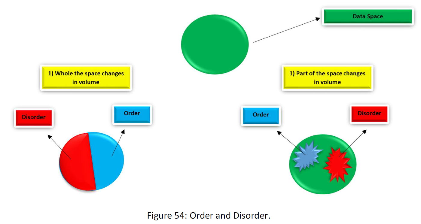
The point is that the volume of the space that it’s volume decreases (order) is equal with the volume of the space that it’s volume decreases (disorder).

I think that could be a good definition of the notion order in general.

The order is the characters within a data to be compressed based on a theory (Set of commands)

It seems right. Suppose the shapes we say that they have order, circle, rectangle etc. They all are capable to be compressed or summarised by their definition. Or in a scientific theory, physics or anything else. We give a set of observations(data) a characteristic in common (command) as a general rule like the rule of gravity( Gm1m2/(r^2) ). And then we claim that we have made them ordered or found in them order. As if scientific theories make just what we observe(data) summarized(compressed). 

But there is an important point:

No theory can make all possible worlds ordered, and if it makes part of them ordered, will make another part disordered.

The above claim seems inevitable. If there is so, how our scientific theories work? What is the benefit to them?

There are two possible answers for them.

1) our world doesn’t contain all possible conditions, and thus we are not opposed to all the space. We just oppose with part of the space (the blue part), and our theories make the part (the part that exists in reality) ordered or compressed and also makes the part that doesn’t exist, disordered and decompressed. In this way, science is a try to find the true glasses, set of commands, conversion or compress method to make the part of the nature that exists ordered.

But the point is that through time the nature changes. The possibilities or arrays that don’t exist come into being and the question is:

Does any theory can maintain through conversions of time.

That is another time, things come into being that wasn’t at first, and data that were in the disordered area (red part) come into the set of data that exist. Then, can any theory maintain the changes? That’s a question worthy to think about.

2) another answer is that the world contains all possible conditions. (like what physicists say about possible worlds) 

In this way we can say: 

there is no true theory.

End